Automatic detection and observation of mineral extraction sites in Switzerland

Clémence Herny (Exolabs), Shanci Li (Uzufly), Alessandro Cerioni (État de Genève), Roxane Pott (swisstopo)

Proposed by swisstopo - PROJ-DQRY-TM
October 2022 to February 2023 - Published on January 2024

Abstract: Studying the evolution of mineral extraction sites (MES) is of primary importance for assessing the availability of mineral resources, managing MES and evaluating the impact of mining activity on the environment. In Switzerland, MES are inventoried at local level by the cantons and at federal level by swisstopo. The latter performs manual vectorisation of MES boundaries. Unfortunately, although the data is of high quality, it is not regularly updated. To automate this tedious task and to better observe the evolution of MES, swisstopo has solicited the STDL to carry out an automatic detection of MES in Switzerland over the years. We performed instance segmentation using a deep learning method to automatically detect MES in RGB aerial images with a spatial resolution of 1.6 m px^-1. The detection model was trained with 266 labels and orthophotos from the SWISSIMAGE RGB mosaic published in 2020. The selected trained model achieved a f1-score of 82% on the validation dataset. The model was used to do detection by inference of potential MES in SWISSIMAGE RGB orthophotos from 1999 to 2021. The model shows good ability to detect potential MES with about 82% of labels detected for the 2020 SWISSIMAGE mosaic. The detections obtained with SWISSIMAGE orthophotos acquired over different years can be tracked to observe their temporal evolution. The framework developed can perform detection in an area of interest (about a third of Switzerland at the most) in just a few hours, which is a major advantage over manual mapping. We acknowledge that there are some missed and false detections in the final product, and the results need to be reviewed and validated by domain experts before being analysed and interpreted. The results can be used to perform statistics over time and update MES evolution in future image acquisitions.

1. Introduction

1.1 Context

Mineral extraction constitutes a strategic activity worldwide, including in Switzerland. Demand for mineral resources has been growing significantly in recent decades¹, mainly due to the rapid increase in the production of batteries and electronic chips, or buildings construction, for example. As a result, the exploitation of some resources, such as rare earth elements, lithium, or sand, is putting pressure on their availability. Being able to observe the development of mineral extraction sites (MES) is of primary importance to adapting mining strategy and anticipating demand and shortage. Mining has also strong environmental and societal impact²³. It implies the extraction of rocks and minerals from water ponds, cliffs, and quarries. The surface affected, initially natural areas, can reach up to thousands of square kilometres¹. The extraction of some minerals could lead to soil and water pollution and involves polluting truck transport. Economic and political interests of some resources might overwhelm land protection, and conflicts are gradually intensifying².

MES are dynamic features that can evolve according to singular patterns, especially if they are small, as is the case in Switzerland. A site can expand horizontally and vertically or be filled to recover the site⁴²³⁵. Changes can happen quickly, in a couple of months. As a results, updating the MES inventory can be challenging.
There is a significant demand for effective MES observation of development worldwide. Majority of MES mapping is performed manually by visual inspection of images¹. Alternatively, recent improvements in the availability of high spatial and temporal resolution space/airborne imagery and computational methods have encouraged the development of automated image processing. Supervised classification of spectral images is an effective method but requires complex workflow ⁶⁴². More recently, few studies have implemented deep learning algorithms to train models to detect extraction sites in images and have shown high levels of accuracy³.

In Switzerland, MES management is historically regulated on a canton-based level using GIS data, including information about the MES location, extent, and extracted materials among others. At the federal level, swisstopo and the Federal Office of Statistics (FSO) observe the development of MES. swisstopo has carried out a detailed manual delineation of MES based on SWISSIMAGE dataset over Switzerland.

In the scope to fasten and improving the process of MES mapping in Switzerland, we developed a method for automating MES detection over the years. Ultimately, the goal is to keep the database up to date when new images are acquired. The results can be statistically process to better assess the MES evolution over time in Switzerland.

1.2. Approach

The STDL has developed a framework named object-detector to automatically detect objects in a georeferenced imagery dataset based on deep learning method. The framework can be adapted to detect MES (also referred as quarry in the project) in Switzerland.

A project to automatically detect MES in Switzerland⁷ has been carried out by the STDL in 2021 (detector-interface framework). Detection of potential MES obtained by automatic detection on the 2020 SWISSIMAGE mosaic has already been delivered to swisstopo (layer 2021_10_STDL_QC1). The method has proven its efficiency detecting MES. The numerical model trained with the object detector achieved a f1-score of 82% and detected about 1200 potential MES over Switzerland.

In this project, we aim to continue this work and extend it to a second objective, that of observing MES evolution over time. The main challenge is to prove the algorithm reliability for detecting objects in a multi-year dataset images acquired with different sensors.

The project workflow is synthesised in Figure 1. First, a deep learning algorithm is trained using a manually mapped MES dataset that serves as ground truth (GT). After evaluating the performance of the trained model, the selected one was used to perform inference detection for a given year dataset and area of interest (AoI). The results were filtered to discard irrelevant detection. The operation was repeated over several years. Finally, each potential MES detected was tracked over the years to observe its evolution.

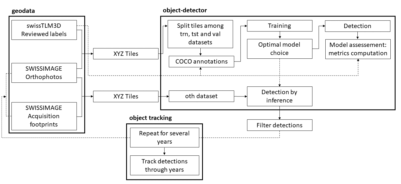
Figure 1: Workflow diagram for automatic MES detection.

In this report, we first describe the data used, including the image description and the definition of AoI. Then we explain the model training, evaluation and object detection procedure. Next, we present the results of potential MES detection and the MES tracking strategy. Finally, we provide conclusion and perspectives.

2. Data

2.1 Images and area of interest

Automatic detection of potential MES over the years in Switzerland was performed with aerial orthophotos from the swisstopo product SWISSIMAGE Journey. Images are georeferenced RGB TIF tiles with a size of 256 x 256 pixels (1 km²).

Product	Year	Coordinate system	Spatial resolution
SWISSIMAGE 10 cm	2017 - current	CH1903+/MN95 (EPSG:2056)	0.10 m (\(\sigma\) \(\pm\) 0.15 m) - 0.25 m
SWISSIMAGE 25 cm	2005 - 2016	MN03 (2005 - 2007) and MN95 (since 2008)	0.25 m (\(\sigma\) \(\pm\) 0.25 m) - 0.50 m (\(\sigma\) \(\pm\) 3.00 - 5.00 m)
SWISSIMAGE 50 cm	1998 - 2004	MN03	0.50 m (\(\sigma\) \(\pm\) 0.50 m)

Table 1: SWISSIMAGE products characteristics.

Several SWISSIMAGE products exist, produced from different instrumentation (Table 1). SWISSIMAGE mosaics are built and published yearly. The year of the mosaic corresponds to the last year of the dataset publication, and the most recent orthophotos datasets available are then used to complete the mosaic. For example the 2020 SWISSIMAGE mosaic is a combination of 2020, 2019 and 2018 images acquisition. The 1998 mosaic release corresponds to a year of transition from black and white images (SWISSIMAGE HIST) to RGB images. For this study, only RGB data from 1999 to 2021 were considered.

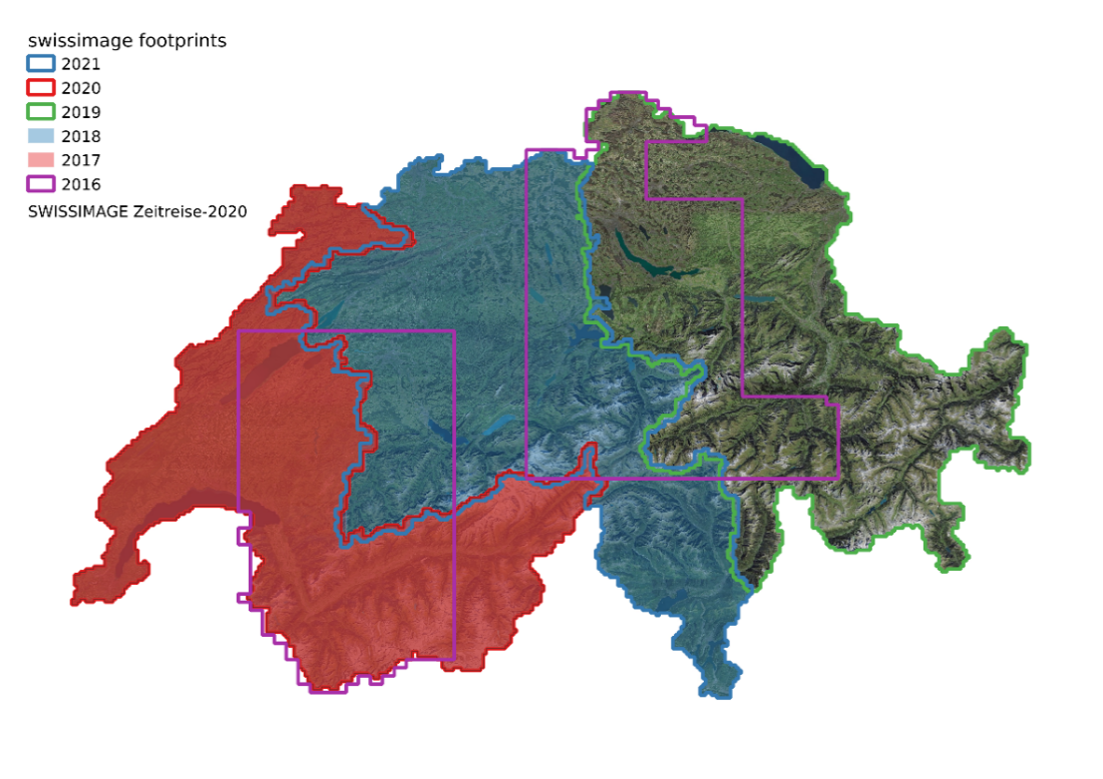
Figure 2: Acquisition footprint of SWISSIMAGE aerial orthophotos for the years 2016 to 2021. The SWISSIMAGE Journey mosaic in the background is the 2020 release.

Acquisition footprints of yearly acquired orthophotos were used as AoI to perform MES detection through time. Over the years, the footprints may spatially overlap (Fig. 2). Since 2017, the geometry of the acquisition footprints has been quasi-constant, dividing Switzerland into three more or less equal areas, ensuring that the orthophotos are updated every three years. For the years before 2017, the acquisition footprints were not systematic and do not guarantee a periodically update of the orthophotos. The acquisition footprint may also not be spatially contiguous.

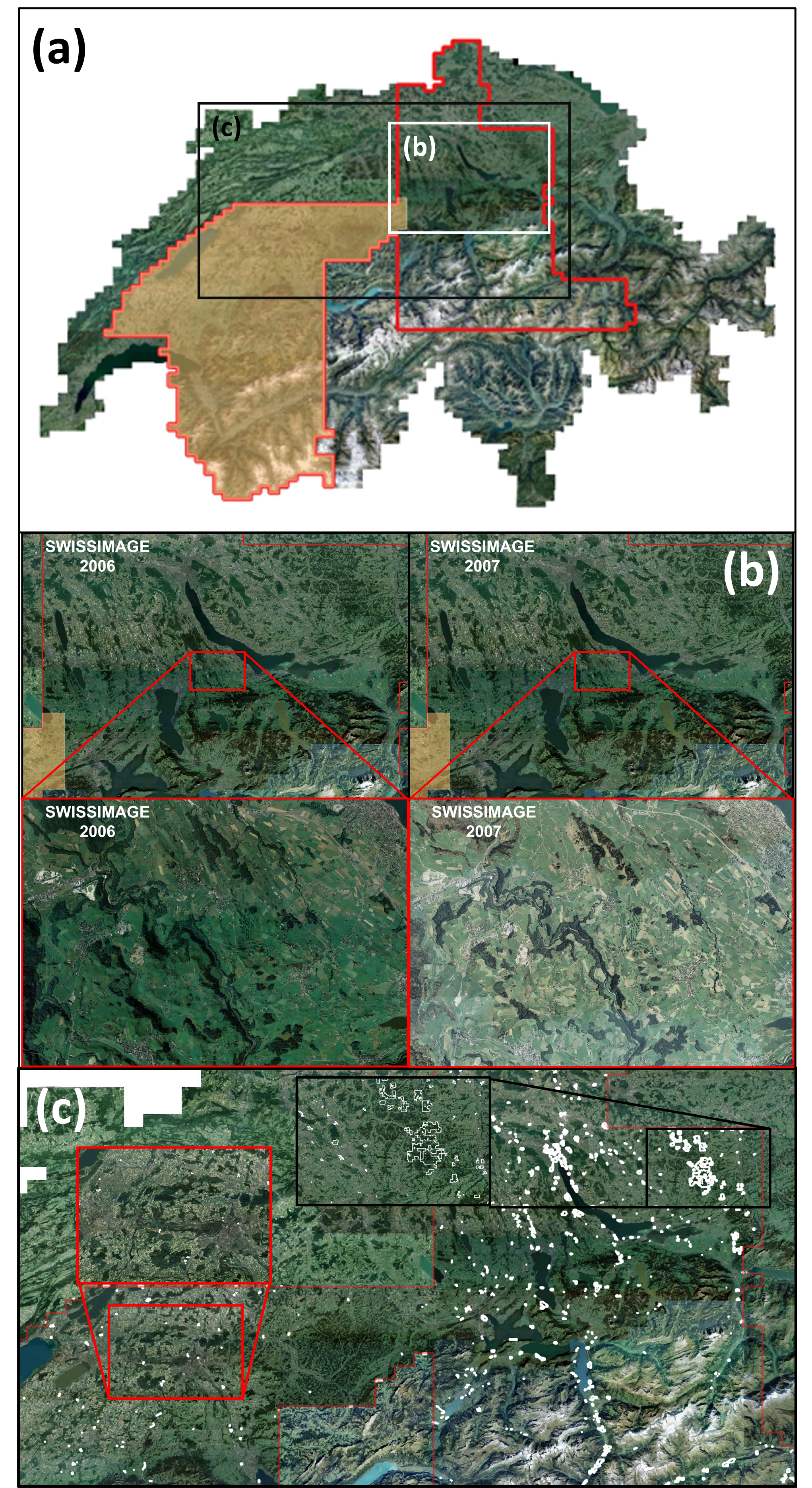
Figure 3: Illustration of the combination of SWISSIMAGE images and FSO images for the 2007 SWISSIMAGE mosaic. (a) Overview of the 2007 SWISSIMAGE mosaic. The red polygon corresponds to the provided SWISSIMAGE acquisition footprint for 2007. The orange polygon corresponds to the surface covered by the new SWISSIMAGE for 2007. The remaining area of the red polygon corresponds to the FSO image dataset acquired in 2007. The black box indicates the panel (b) location, and the white box indicates the panel (c) location. (b) Side-by-side comparison of image composition in 2006 and 2007 SWISSIMAGE mosaics. (c) Examples of detection polygons (white polygons) obtained by inference on the 2007 SWISSIMAGE dataset (red box) and FSO images 2007 (outlined by black box).

SWISSIMAGE Journey mosaics of 2005, 2006, and 2007 present a particularity as it is composed not only of 25 cm resolution SWISSIMAGE but also of orthophotos acquired for the FSO. These are tiff RGB orthophotos with a spatial resolution of 50 cm px^-1 (coordinate system: CH1903/LV03 (EPSG:21781)) and have been integrated into the SWISSIMAGE Journey products. However, these images were discarded (modification of the footprint shape) from our dataset because they were causing issues in the MES automatic detection producing odd segmented detection shapes (Fig. 3). This is probably due to the different stretching of pixel colour between datasets.

It also has to be noted that there are currently missing images (about 88 tiles at zoom level 16) in the 2020 SWISSIMAGE dataset.

2.2 Image fetching

Pre-rendered SWISSIMAGE tiles (256 x 256 px, 1 km²) are downloaded using the Web Map Tile Service (WMTS) wmts.geo.admin.ch via an XYZ connector. Tiles are served on a cartesian coordinates grid using a Web Mercator Quad projection and a coordinate reference system EPGS 3857. Position of a tile on the grid is defined by x and y coordinates and the pixel resolution of the image is defined by z, its zoom level. Changing the zoom level affects the resolution by a factor of 2 (Fig. 4). For instance a zoom level of 17 corresponds to a resolution of 0.8 m px^-1 and a zoom level of 16 to a resolution of 1.6 m px^-1.

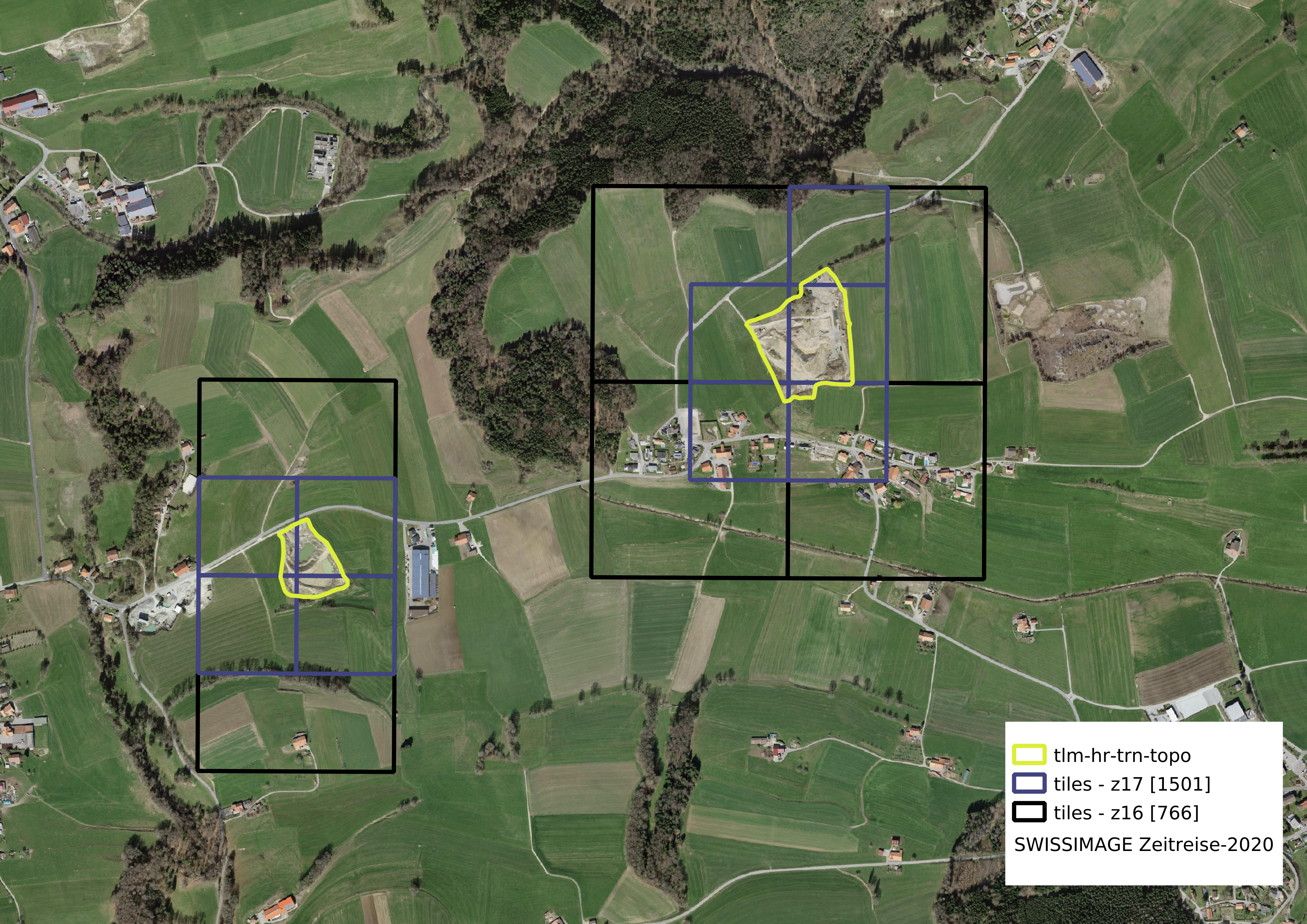
Figure 4: Examples of tiles geometry at zoom level 16 (z16, black polygons) and at zoom level 17 (z17, blue polygons). The number of tiles for each zoom level is indicated in square brackets. The tiles are selected for model training, i.e. only tiles intersecting swissTLM3D labels (tlm-hr-trn-topo, yellow polygons).

Note that in the subsequent project carried out by Reichel and Hamel (2021)⁷, the tiling method adopted was slightly different from the one adopted for this project. Custom size and resolution tiles were built. A sensitivity analysis of these two parameters was conducted and led to the choice of tiles with a size of about 500 m and a pixel resolution of about 1 m (above, the performance was not significantly improved).

2.3 Ground truth

The MES labels originate from the swiss Topographic Landscape Model 3D (swissTLM3D) produced by swisstopo. swissTLM3D is a large-scale topographic landscape model of Switzerland, including manually drawn and georeferenced vectors of objects of interest at a high resolution, including MES features. Domain experts from swisstopo have carried out extensive work to review the labeled MES and to synchronise them with the 2020 SWISSIMAGE mosaic to improve the quality of the labeled dataset. A total of 266 labels are available. The mapped MES reveal the diversity of MES characteristics, such as the presence or absence of buildings/infrastructures, trucks, water pounds, and vegetation (Fig. 5).

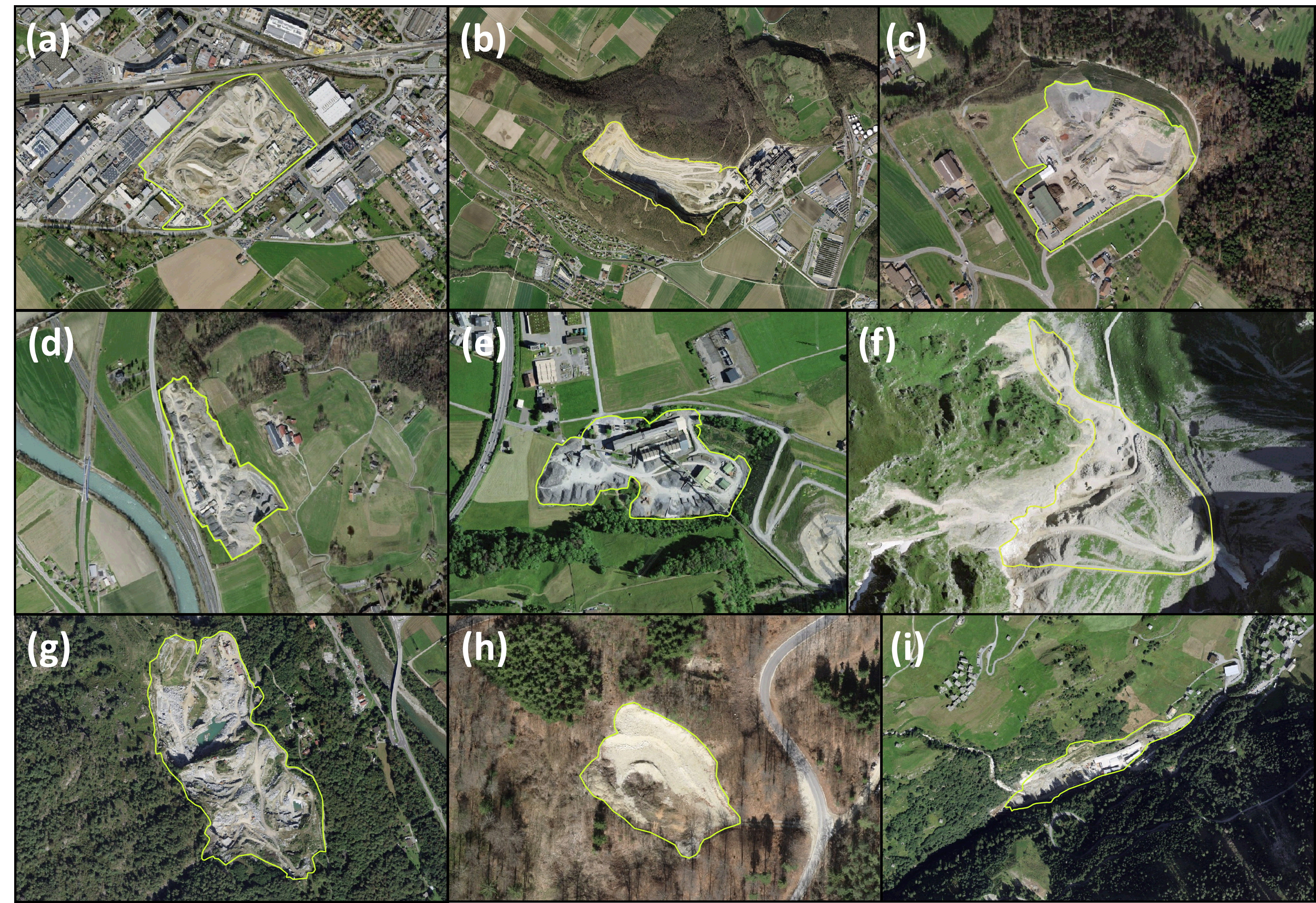
Figure 5: Examples of MES mapped in swissTLM3D and synchronised to 2020 SWISSIMAGE mosaic.

These labels are used as the ground truth (GT) i.e. the reference dataset indicating the presence of a MES in an image. The GT is used both as input to train the model to detect MES and to evaluate the model performance.

3. Automatic detection methodology

3.1 Deep learning algorithm for object detection

Training and inference detection of potential MES in SWISSIMAGE were performed with the object detector framework. This project is based on the open source detectron2 framework⁸ implemented with PyTorch by the Facebook Artificial Intelligence Research group (FAIR). Instance segmentation (delineation of object) was performed with a Mask R-CNN deep learning algorithm⁹. It is based on a Recursive-Convolutional Neural Network (CNN) with a backbone pre-trained model ResNet-50 (50 layers deep residual network).

Images were annotated with custom COCO object based on the labels (class 'Quarry'). The model is trained with this dataset to later perform inference detection on images. If the object is detected by the algorithm, a pixel mask is produced with a confidence score (0 to 1) attributed to the detection (Fig. 6).

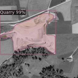
Figure 6: Example of detection mask. The pink rectangle corresponds to the bounding box of the object, the object is segmented by the pink polygons associated with the detection class ('Quarry') and a confidence score.

The object detector framework permits to convert detection mask to georeferenced polygon that can be used in GIS softwares. The implementation of the Ramer-Douglas-Peucker (RDP) algorithm, allows the simplification of the derived polygons by discarding non-essential points based on a smoothing parameter. This allow to considerably reduces the amount of data to be stored and prevent potential memory saturation while deriving detection polygons on large areas as it is the case for this study.

3.2 Model training

Orthophotos from the 2020 SWISSIMAGE mosaic, for which the GT has been defined, were chosen to proceed the model training. Tiles intersecting labels were selected and split randomly into three datasets: the training dataset (70%), the validation dataset (15%), and the test dataset (15%). Addition of empty tiles (no annotation) to confront the model to landscapes not containing the target object has been tested (Appendix A.1) but did not provide significant improvement in the model performance to be adopted.

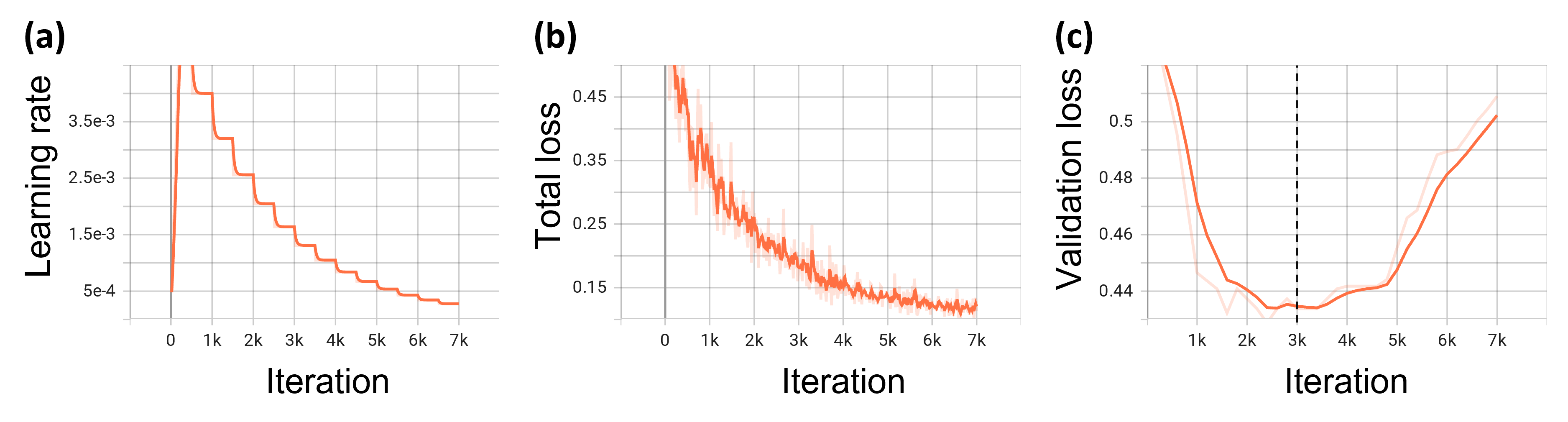
Figure 7: Training curves obtained at zoom level 16 on the 2020 SWISSIMAGE mosaic. The curves were obtained for the trained model 'replicate 3'. (a) Learning rate in function of iteration. The step was defined every 500 iterations. The initial learning rate was 5.0 x 10^-3 with a weight and bias decay of 1.0 x 10^-4. (b) The total loss is a function of iteration. Raw measurement (light red) and smoothed curve (0.6 factor, solid red) are superposed. (c) The validation loss curve is a function of iteration. Raw measurement (light red) and smoothed curve (0.6 factor, solid red) are superposed. The vertical dashed black lines indicate the iteration minimising the validation loss curve, i.e. 3000.

Models were trained with two images per batch (Appendix A.2), a learning rate of 5 x 10^-3, and a learning rate decay of 1 x 10^-4 every 500 steps (Fig. 7 (a)). For the given model, parameters and a zoom level of 16 (Section 3.3.3), the training is performed over 7000 iterations and lasts about 1 hour on a 16 GiB GPU (NVIDIA Tesla T4) machine compatible with CUDA. The total (train and validation loss) loss curve decreases until reaching a quasi-steady state around 6000 iterations (Fig. 7 (b)). The optimal detection model corresponds to the one minimising the validation loss curve. This minimum is reached between 2000 and 3000 iterations (Fig. 7 (c)).

3.3 Metrics

The model performance and detection reliability were assessed by comparing the results to the GT. The detection performed by the model can be either (1) a True Positive (TP), i.e. the detection is real (spatially intersecting the GT) ; (2) a False Positive i.e. the detection is not real (not spatially intersecting the GT) or (3) a False Negative (FN) i.e. the labeled object is not detected by the algorithm (Fig. 8). Tagging the detection (Fig. 9(a)) allows to calculate several metrics (Fig. 9(b)) such as:

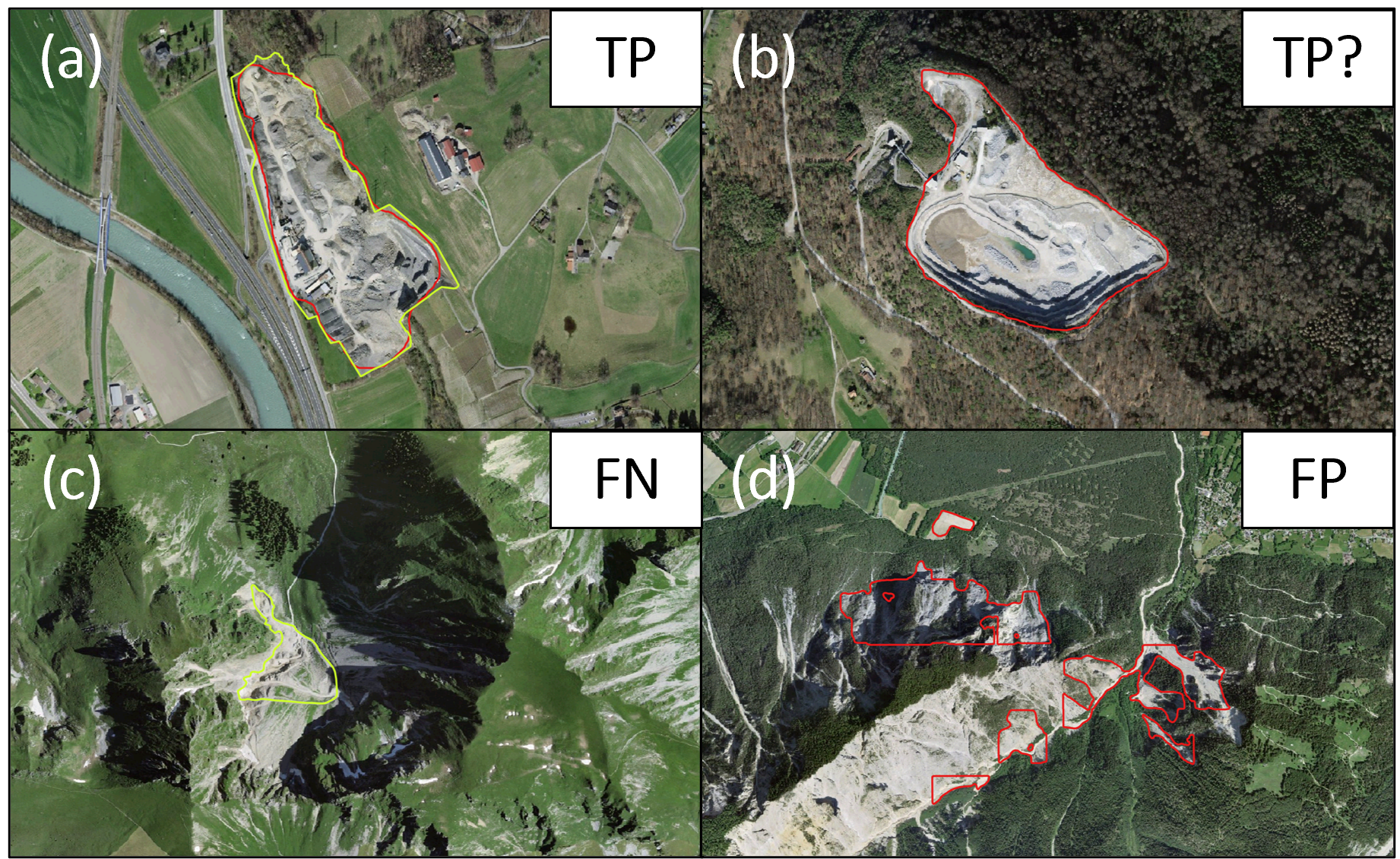
Figure 8: Examples of different detection cases. Label is represented with a yellow polygon and detection with a red polygon. (a) True Positive (TP) detection intersecting the GT, (b) a potential True Positive (TP?) detection with no GT, (c) False Negative (FN) case with no detection while GT exists, (d) False Positive (FP) detection of object that is not a MES.

• the recall, translating the amount of TP detections predicted by the model:

  \[recall = \frac{TP}{(TP + FN)}\]

• the precision, translating the number of well-predicted TP among all the detections:

  \[precision = \frac{TP}{(TP + FP)}\]

• the f1-score, the harmonic average of the precision and the recall:

  \[f1 = 2 \times \frac{recall \times precision}{recall + precision}\]

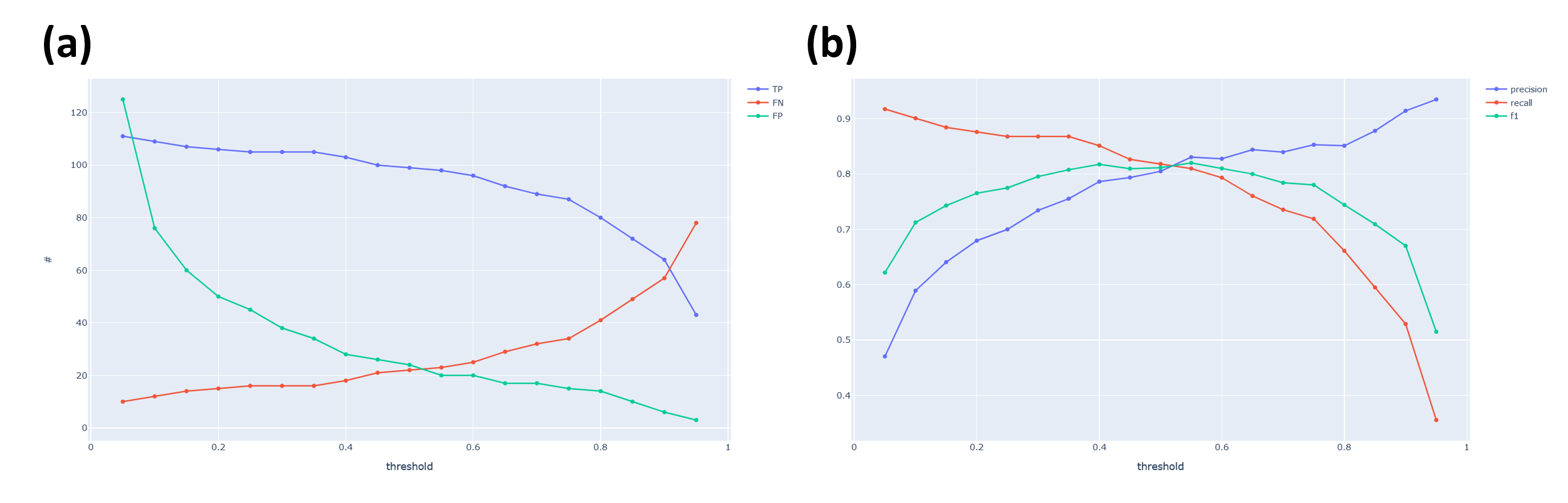
Figure 9: Evaluation of the trained model performance obtained at zoom level 16 for the trained model 'replicate 3' (Table 2). (a) Number of TP (blue), FN (red), and FP (green) as a function of detection score threshold for the validation dataset. (b) Metrics value, precision (blue), recall (red), and f1-score (green) as a function of the detection score threshold for the validation dataset. The maximum f1-score value is 82%.

4. Automatic detection model analysis

4.1. Model performance and replicability

Trained models reached f1-scores of about 80% with a standard deviation of 2% (Table 2). The performances are similar to the model trained by Reichel and Hamel (2021)⁷.

model	precision	recall	f1
replicate 1	0.84	0.79	0.82
replicate 2	0.77	0.76	0.76
replicate 3	0.83	0.81	0.82
replicate 4	0.89	0.77	0.82
replicate 5	0.78	0.82	0.80

Table 2: Metrics value computed for the validation dataset for trained models replicates with the 2020 SWISSIMAGE mosaic at zoom level 16.

A variability is expected as the deep learning algorithm displays some random behavior, but it is supposed to be negligible. However, the observed model variability is enough to affect final results that might slightly change by using different trained models with same input parameters (Fig. 10).

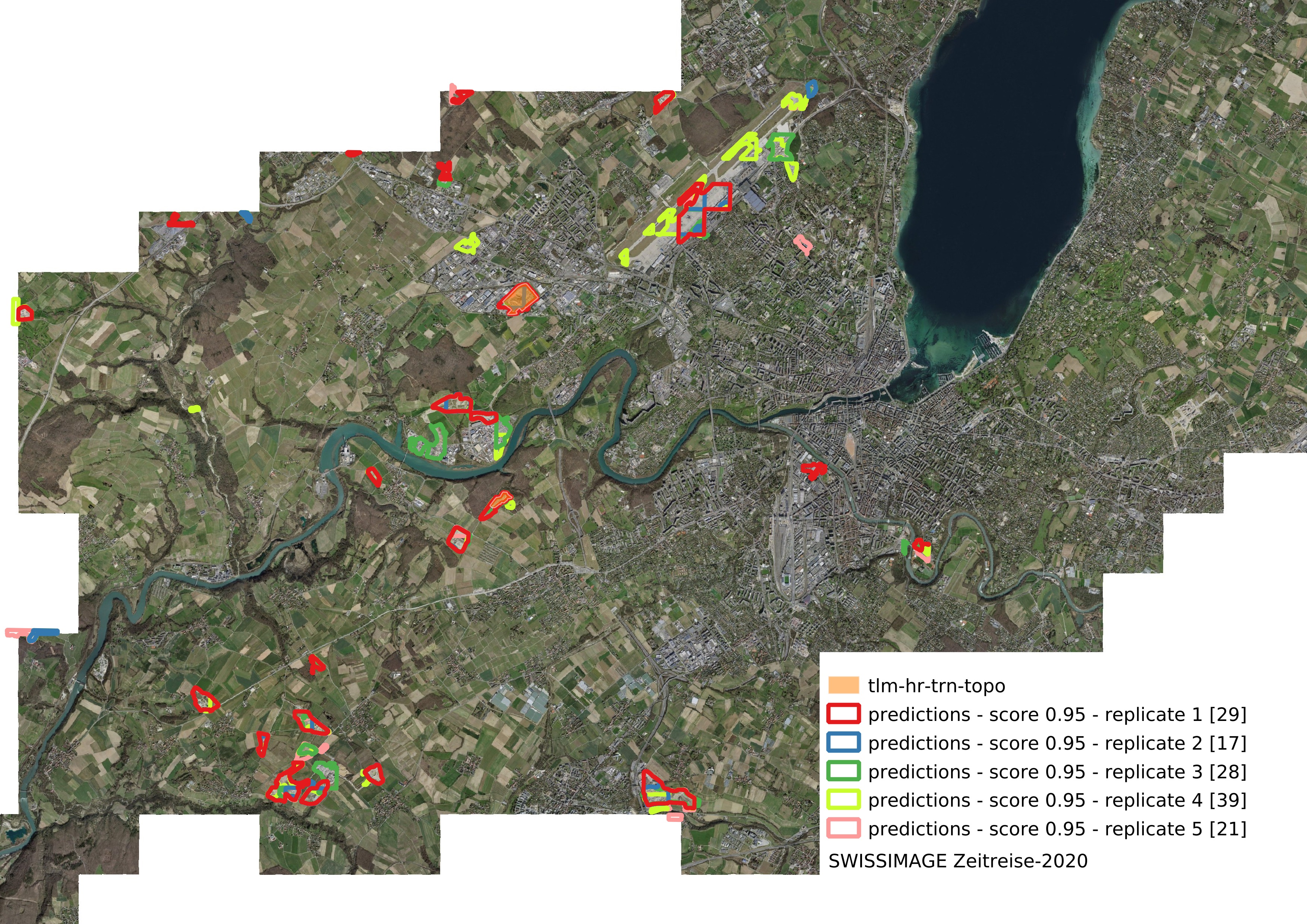
Figure 10: Detection polygons obtained for the different trained model replicates (Table 2) highlighting results variability. The labels correspond to orange polygons. The number in the square bracket corresponds to the number of polygons. The inference detections have been performed on a subset of 2000 tiles for the 2020 SWISSIMAGE at zoom level 16. Detections have been filtered according to the parameters defined in Section 5.1.

To reduce the variability of the trained models, the random seeds of both detectron2 and python have been fixed. Neither of these attempts have been successful, and the variability remains. The nondeterministic behavior of detectron2 has been recognised (issue 1, issue 2), but no suitable solution has been provided yet. Further investigation on the model performance and consistency should be performed in the future.

To mitigate the results variability of model replicates, we could consider in the future to combine the results of several model replicates to remove FP while preserving the TP and potential TP detection. The choice and number of models used should be evaluated. This method is tedious as it requires inference detection from several models, which can be time-consuming and computationally intensive.

4.2 Sensitivity to the zoom level

Image resolution is dependent on the zoom level (Section 2.2). To select the most suitable zoom level for MES detection, we performed a sensitivity analysis on trained model performance. Increasing the zoom level increases the value of the metrics following a global linear trend (Fig. 11).

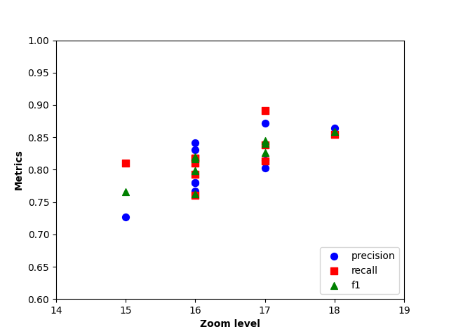
Figure 11: Metrics values (precision, recall and f1) as function of zoom level for the validation dataset. The results of the replicates performed at each zoom level are included (Table A1).

Models trained at a higher zoom level performed better. However, a higher zoom level implies smaller tile and thus, a larger number of tiles to fill the AoI. For a typical AoI, i.e up to a third of Switzerland, this can lead to a large number of tiles to be stored and processed, leading to potential RAM and/or disk space saturation. For 2019 AoI, 89'290 tiles are required at zoom level 16 while 354'867 tiles are required at zoom level 17, taking respectively 3 hours and 11 hours to process on a 30 GiB RAM machine with a 16 GiB GP.

Visual comparison of inference detection reveals that there was no significant improvement in the object detection quality from zoom level 16 to zoom level 17. Both zoom level present a similar proportion of detections intersecting labels (82% and 79% for zoom level 16 and zoom level 17 respectively). On the other hand, the quality of object detection at zoom level 15 was depreciated. Indeed, detection scores were lower, with only tens of detection scores above 0.95 while it was about 400 at zoom level 16 and about 64% of detection intersecting labels.

4.3 Model choice

Based on tests performed, we selected the 'replicate 3' model, obtained (Tables 2 and A1) at zoom level 16, to perform inference detection.

Models trained at zoom level 16 (1.6 m px^-1 pixel resolution) have shown satisfying results in accurately detecting MES contour and limiting the number of FP with high detection score (Fig. 11). It represents a good trade-off between results reliability (f1-score between 76% and 82% on the validation dataset) and computational resources.
Then, among all the replicates performed at zoom level 16, we selected the trained model 'replicate 3' (Table 2) because it combines both the highest metrics values (for the validation dataset but also the train and test datasets), close precision and recall values and a rather low amount of low score detections.

5. Automatic detection of MES

5.1 Detection post-processing

Detection by inference was performed over AoIs with a threshold detection score of 0.3 (Fig. 12). The low score filtering results in a large amount of detections. Several detections may overlap, potentially segmenting a single object. In addition a detection might be split into multiple tiles. To improve the pertinence and the aesthetics of the raw detection polygons, a post-processing procedure was applied.

First, a large proportion of FP occurred in mountainous areas (rock outcrops and snow, Fig. 12(a)). We assumed MES are not present (or at least sparse) above a given altitude. An elevation filtering was applied using a Switzerland Digital Elevation Model (about 25 m px^-1) derived from the SRTM instrument (USGS - SRTM). The maximum elevation of the labeled MES is about 1100 m.

Second, detection aggregation was applied: - polygons were clustered (K-means) according to their centroid position. The method involves setting a predefined number k of clusters. Manual tests performed by Reichel and Hamel (2021)⁷ concluded to set k equal to the number of detection divided by three. The highest detection score was assigned to the clustered detection. This method preserves the final integrity of detection polygons by retaining detection that has potentially a low confidence score but belongs to a cluster with a higher confidence score improving the final segmentation of the detected object. The value of the threshold score must be kept relatively low (i.e. 0.3) when performing the detection to prevent removing too many polygons that could potentially be part of the detected object. We acknowledge that determining the optimal number of clusters by clustering validation indices rather than manual adjustment would be more robust. In addition, exploring other clustering methods, such as DBSCAN, based on local density, can be considered in the future. - score filtering was applied. - spatially close polygons were assumed to belong to the same MES and are merged according to a distance threshold. The averaged score of the merged detection polygons was ultimately computed.

Finally, we assumed that a MES covers a minimal area. Detection with an area smaller than a given threshold were filtered out. The minimum MES area in the GT is 2270 m².

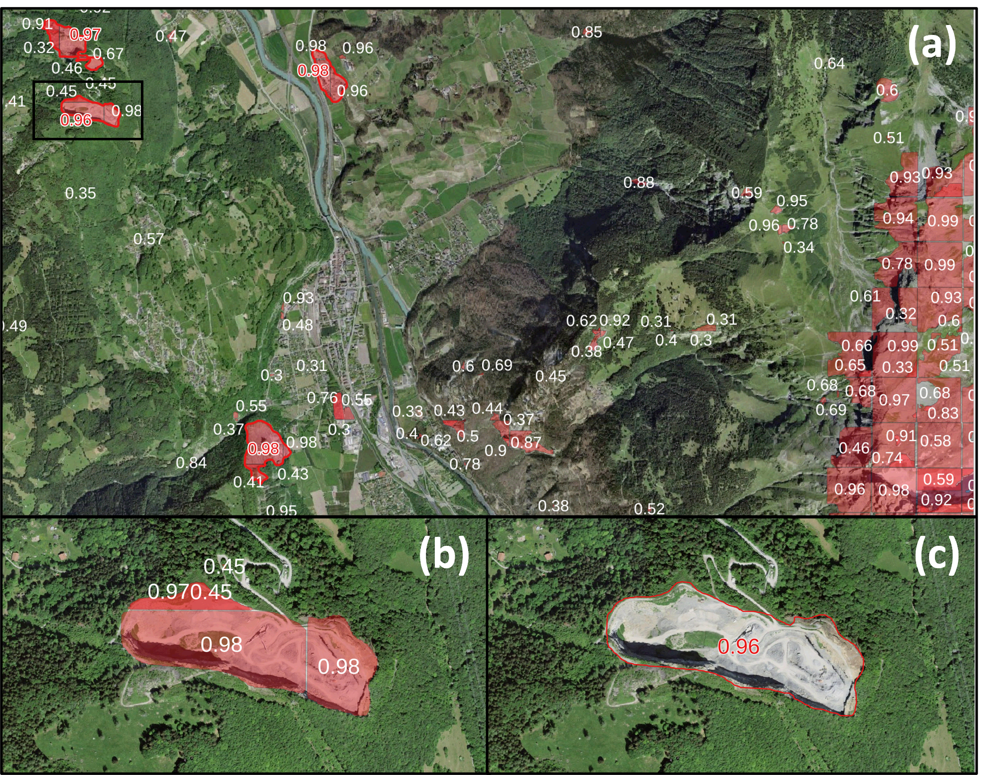
Figure 12: MES detection filtering. (a) Overview of the automatic detection of MES obtained with 2020 SWISSIMAGE at zoom level 16. Transparent red polygons (with associated confidence score in white) correspond to the raw object detection output and the red line polygons (with associated confidence score in red) correspond to the final filtered detection. The black box outlines the location of the (b) and (c) panel zoom. Note the large number of detection in the mountains (right area of the image). (b) Zoom on several raw detections polygons of a single object with their respective confidence score. (c) Zoom on a filtered detection polygon of a single object with the resulting score.

Sensitivity of detections to these filters was investigated (Table 3). The quantitative evaluation of filter combination relevance is tricky as potential MES presence is performed by inference, and the GT provided by swissTLM3D constitutes an incomplete portion of the MES in Switzerland (2020). As indication, we computed the number of spatial intersection between ground truth and detection obtained with the 2020 SWISSIMAGE mosaic. Filter combination number 3 was adopted, allowing to detect about 82% of the GT with a relatively limited amount of FP detection compared to filter combinations 1 and 2 (from visual inspection).

filters combination	score threshold	elevation threshold (m)	area threshold (m2)	distance threshold (m)	number of detection	label detection (%)
1	0.95	2000	1100	10	1745	85.1
2	0.95	2000	1200	10	1862	86.6
3	0.95	5000	1200	10	1347	82.1
4	0.96	2000	1100	10	1331	81.3
5	0.96	2000	1200	8	1445	78.7
6	0.96	5000	1200	10	1004	74.3

Table 3: Threshold values of filtering parameters and their respective number of detections and intersection proportion with swissTLM3D labels. The detections have been obtained for the 2020 SWISSIMAGE mosaic.

We acknowledged that for the selected filter combination, the area threshold value is higher than the smallest area value of the GT polygons. However, reducing the area value increases significantly the presence of FP. Thirteen labels display an area below 5000 m².

5.2 Inference detections

The trained model was used to perform inference detection on SWISSIMAGE orthophotos from 1999 to 2021. The automatic detection model shows good capabilities to detect MES in different years orthophotos (Fig. 13), despite being trained on the 2020 SWISSIMAGE mosaic. The model also demonstrates capabilities to detect potential MES that have not been mapped yet but are strong candidates. However, the model misses some labeled MES or potential MES (FN, Fig. 8). However, when the model process FSO images, with different colour stretching, it failed to correctly detect potential MES (Fig. 3). It reveals that images must have characteristics close to the training dataset for optimal results with a deep learning model.

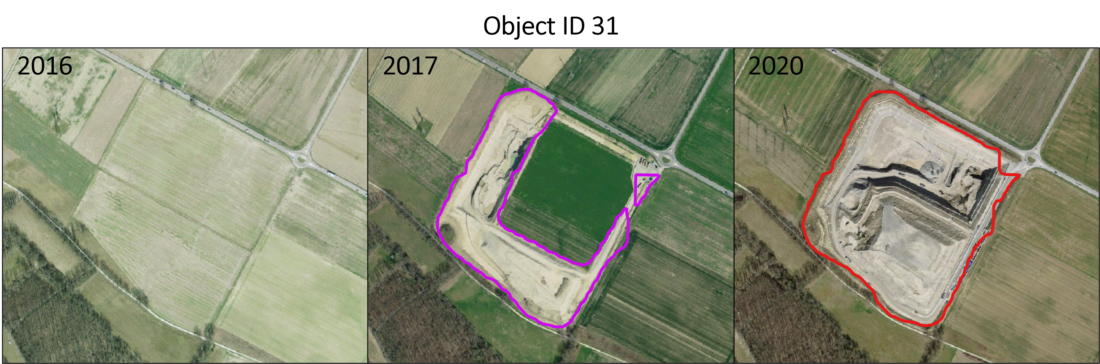
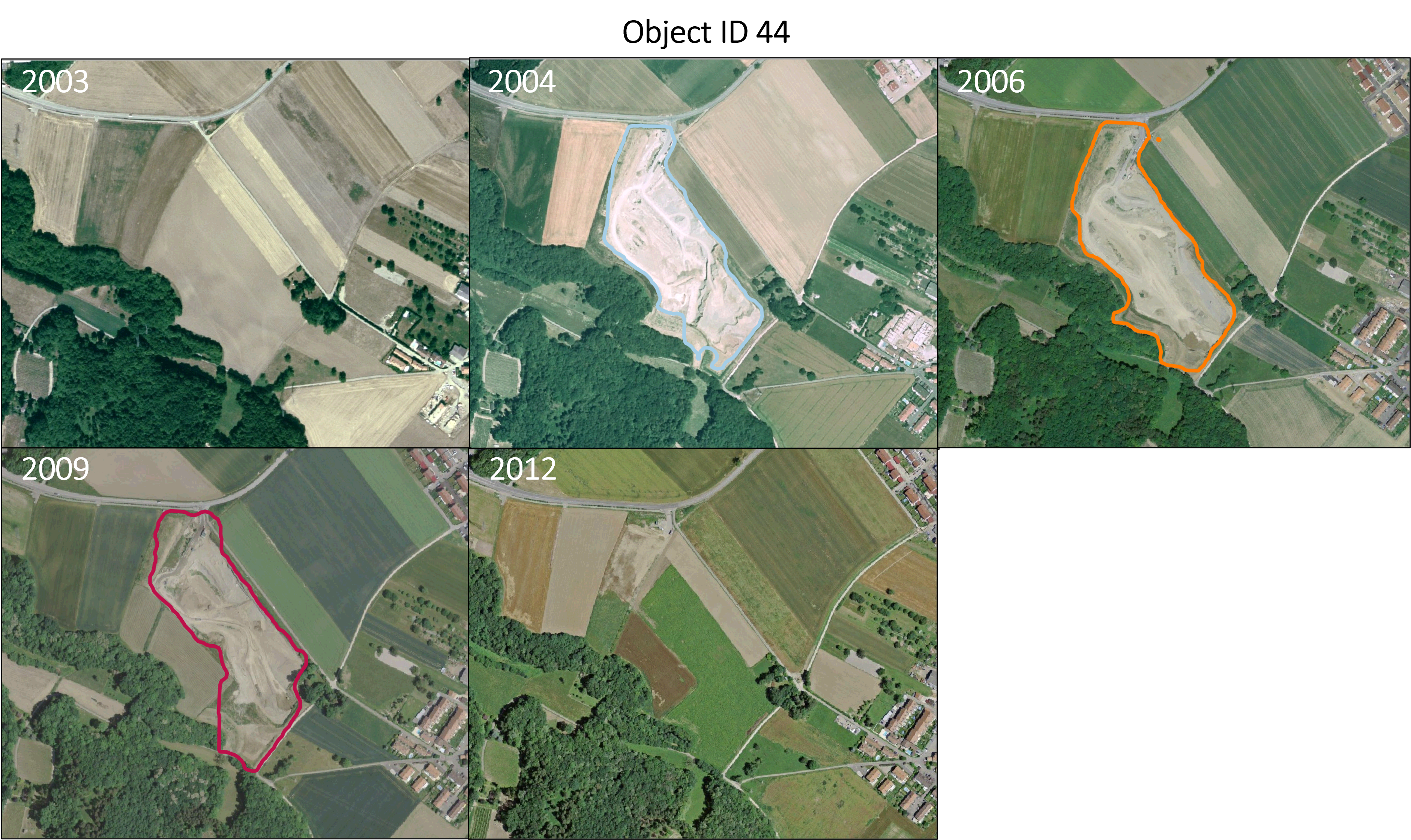
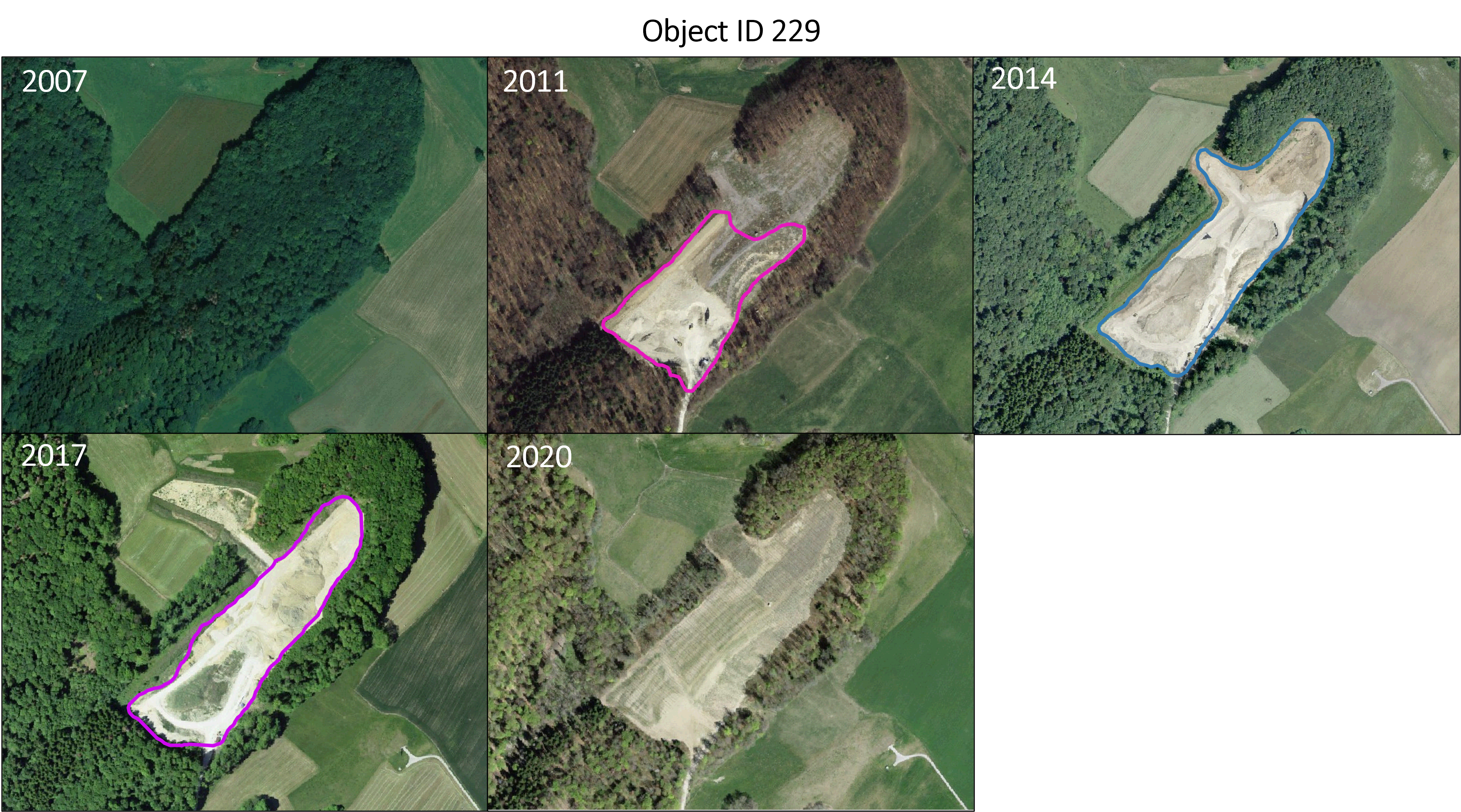
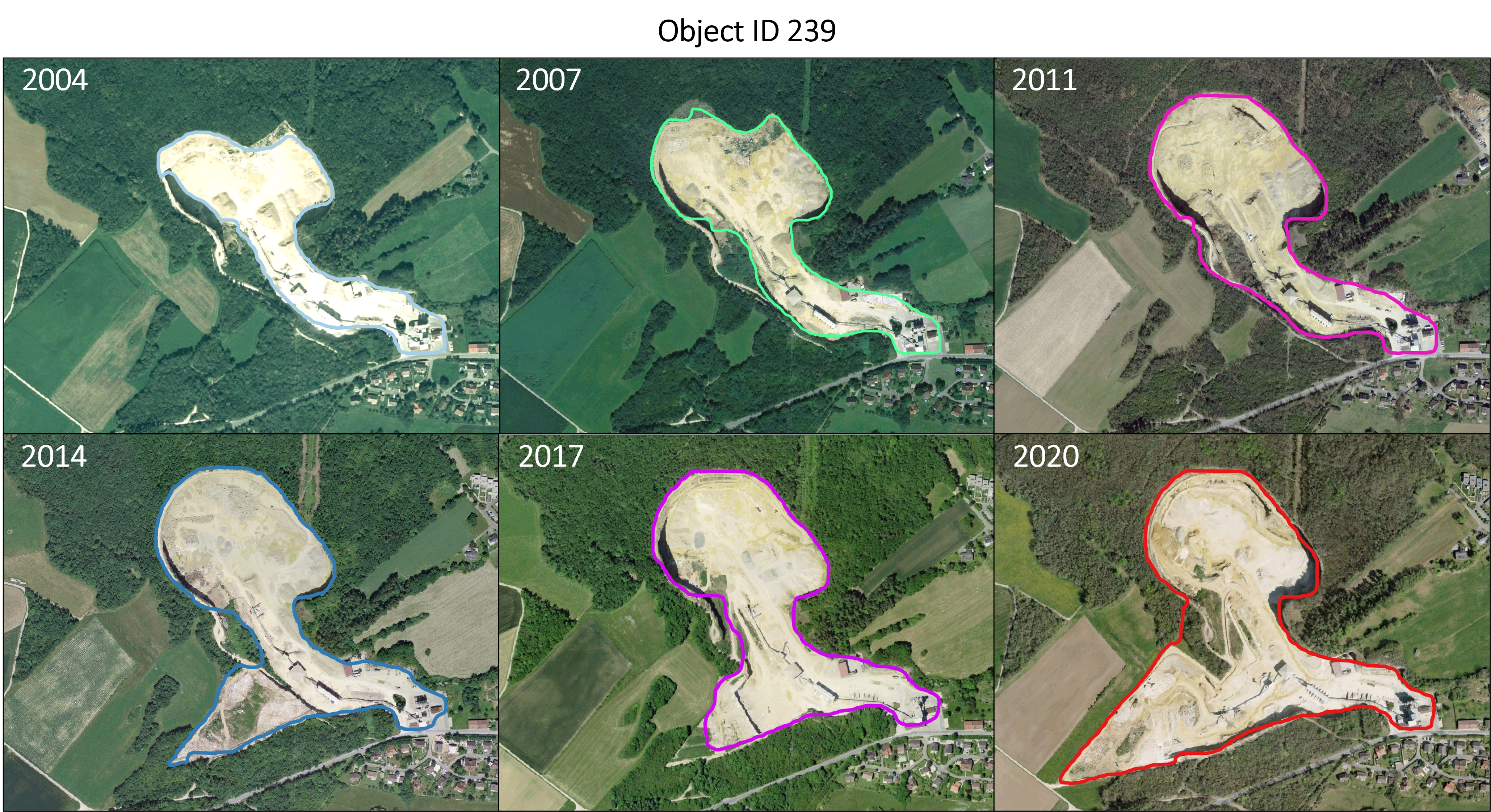
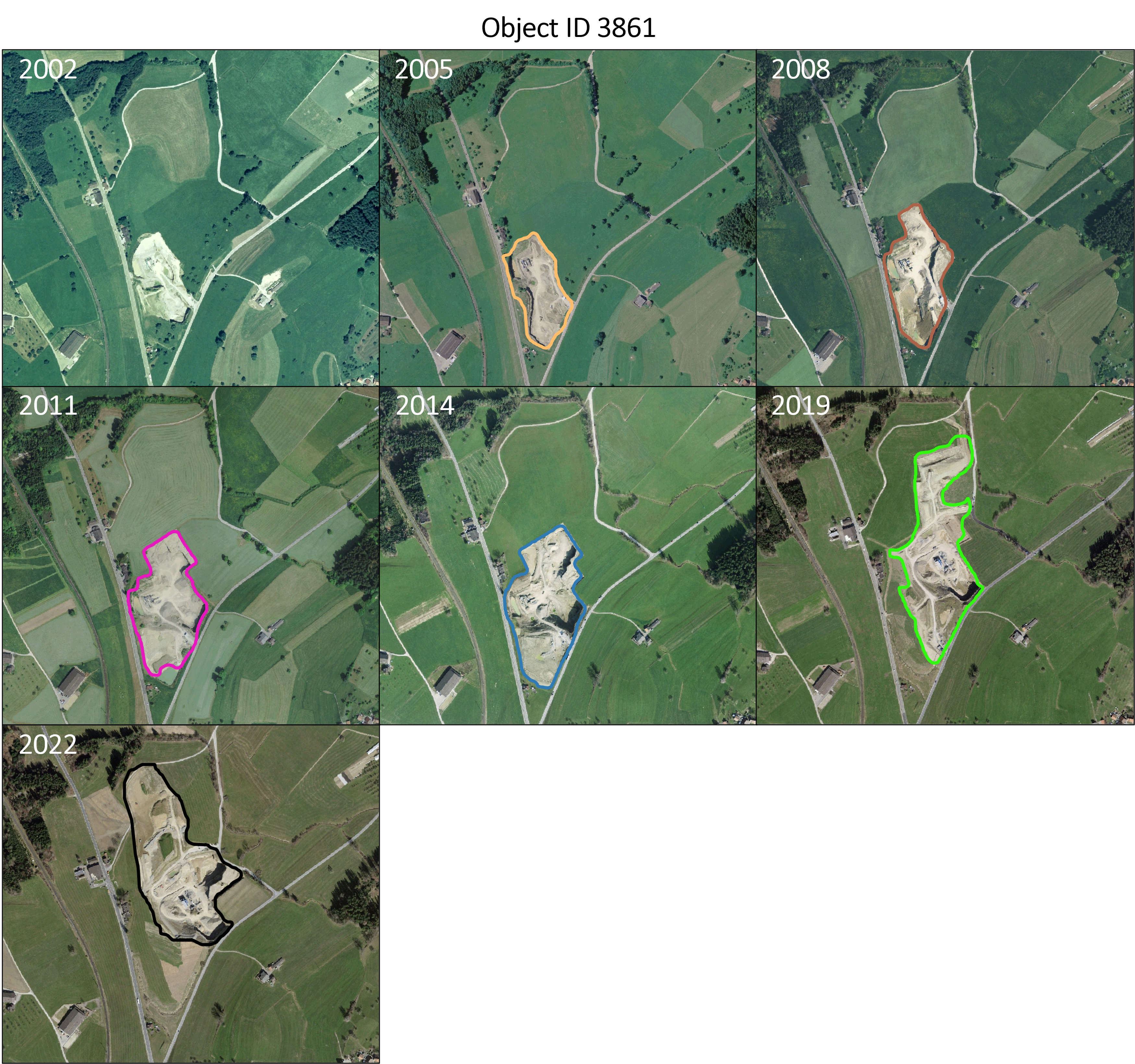Figure 13: Examples of object detection segmented by polygons in different year orthophotos. The yellow polygon for the year 2020 panel of object ID 3761 corresponds to the label. Other coloured polygons correspond to the algorithm detection.

Then, we acknowledge that a significant amount of FP detection can still be observed in our filtered detection dataset (Figs. 8 and 14). The main sources of FP are the presence of large rock outcrops, mountainous areas without vegetation, snow, river sand beds, brownish-coloured fields, or construction areas. MES present a large variety of features (buildings, water pounds, trucks, vegetation) (Fig. 5) which can be a source of confusion for the algorithm but even sometimes for human eye. Therefore, the robustness of the GT is crucial for reliable detection. The algorithm's results should be taken carefully.

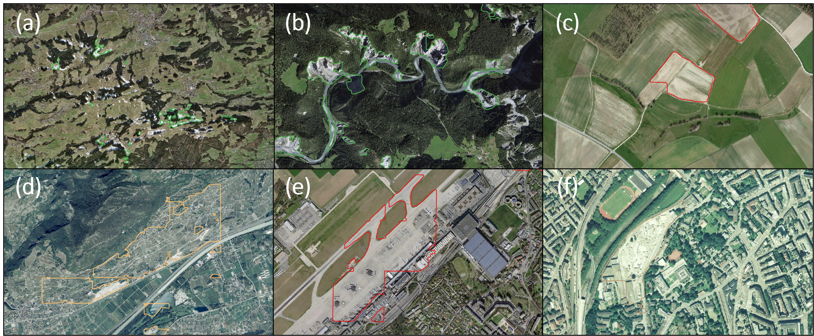
Figure 14: Examples of FP detection. (a) Snow patches (2019) ; (b) River sand beds and gullies (2019); (c) Brownish field (2020); (d) vineyards (2005); (e) Airport tarmac (2020); (f) Construction site (2008).

The detections produced by the algorithm are potential MES, but the final results must be reviewed by experts in the field to discard remaining FP detection and correct FN before any processing or interpretation.

6. Observation of MES evolution

6.1 Object tracking strategy

Switzerland is covered by RGB SWISSIMAGE product over more than 20 years (1999 to actual), allowing changes to be detected (Fig. 13).

Figure 15: Strategy for MES tracking over time. ID assignment to detection. Spatially intersecting polygons share the same ID allowing the MES to be tracked in a multi-year dataset.

We assumed that detection polygons that overlap from one year to another describe a single object (Fig. 15). Overlapping detections and unique detections (which do not overlap with polygons from other years) in the multi-year dataset were assigned a unique object identifier (ID). A new object ID in the timeline indicates: - the first occurrence of the object detected in the dataset of the first year available for the area. It does not mean that the object was not present before, - the creation of a potential new MES.

The disappearance of an object ID indicates its potential refill. Therefore, the chronology of MES, creation, evolution and filling, can be constrained.

6.2 Evolution of MES over years

Figures 13 and 16 illustrate the ability of the trained model to detect and track a single object in a multi-year dataset. The detection over the years appears reliable and consistent, although object detection may be absent from a year dataset (e.g. due to shadows or colour changes in the surroundings). Remember that the image coverage of a given area is not renewed every year. Characteristics of the potential MES, such as surface evolution (extension or retreat), can be quantified. For example, the surfaces of object IDs 239 and 3861 have more than doubled in about 20 years. Tracking object ID along with image visualisation allows observation of the opening and the closing of potential MES, as object IDs 31, 44, and 229.

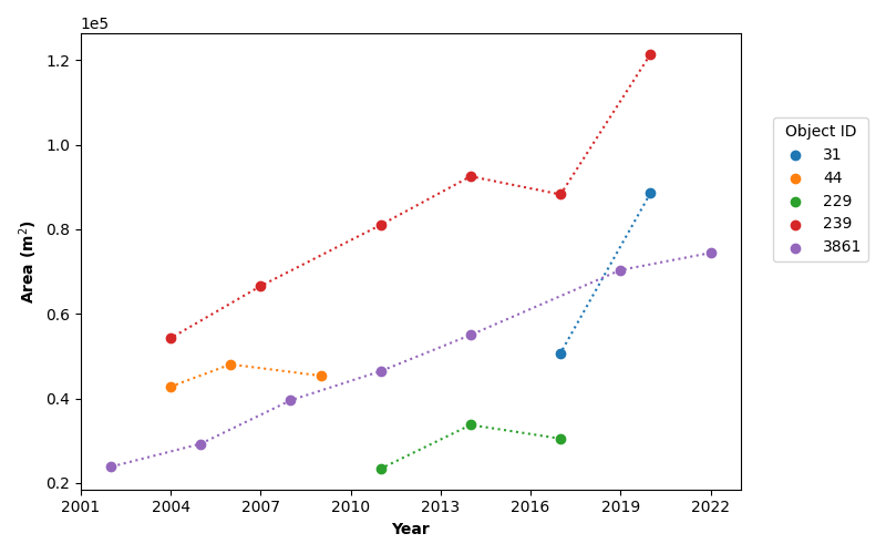
Figure 16: Detection area (m²) as a function of years for several object ID. Figure 13 provides the visualisation of the object IDs selected. Each point corresponds to an object ID occurrence in the corresponding year dataset.

The presence of an object in several years dataset strengthens the likeliness of the detected object to be an actual MES. On the other hand, object detection of only one occurrence is more likely a FP detection.

7. Conclusion and perspectives

The project demonstrated the ability to automatically, quickly (a matter of hours for one AoI), and reliably detect potential MES in orthophotos of Switzerland with an automatic detection algorithm (deep learning). The selected trained model achieved a f1-score of 82% on the validation dataset. The final detection polygons accurately delineate the potential MES. We can track single MES through multiple years, emphasising the robustness of the method to detect objects in multi-year datasets despite the detection model being trained on a single dataset (2020 SWISSIMAGE mosaic). However, image colour stretching different from that used to train the model can significantly affect the model's ability to provide reliable detection, as was the case with the FSO images.

Although the performance of the trained model is satisfactory, FP and FN are present in the datasets. They are mainly due to confusion of the algorithm between MES and rock outcrops, river sandbeds or construction sites. A manual verification of the relevance of the detection by experts in the field is necessary before processing and interpreting the data. Revision of all the detections from 1999 to 2021 is a time-consuming effort but is necessary to guarantee detection reliability. Despite the required manual checks, the provided framework and detection results constitute a valuable contribution that can greatly assist the inventory and the observation of MES evolution in Switzerland. It provides state-wide detection in a matter of hours, which is a considerable time-saving compared with manual mapping. It also enables MES detection with a standardised method, independent of the information or method adopted by the cantons.

Further model improvements could be consider, such as increasing the metrics by improving GT quality, improving model learning strategy, mitigating the model learning variability, or test supervised clustering methods to find relevant detection.

This work can be used to compute statistics to study long-term MES in Switzerland and better management of resources and land use in the future. MES detection can be combined with other data, such as the geologic layer, to identify the mineral/rocks exploited and high-resolution DEM (swissALTI3D) to infer elevation changes and observe excavation or filling of MES⁵.
So far only RGB SWISSIMAGE orthophotos from 1999 to 2021 were processed. Prior to 1999, black and white orthophotos exist but the model trained on RGB images could not be applied trustfully to black and white images. Image colourisation tests (with the help of deep learning algorithm[@farella_colour_2022]) were performed and provided encouraging detection results. This avenue needs to be explored.

Finally, automatic detection of MES is rare¹³, and most studies perform manual mapping. Therefore, the framework could be the extended to other datasets and/or other countries to provide a valuable asset to the community. A global mapping of MES has been completed with over 21'000 polygons¹ and can be used as a GT database to train an automatic detection model.

Code availability

The codes are stored and available on the STDL's github repository:

• proj-dqry: mineral extraction site framework
• object-detector: object detector framework

Acknowledgements

This project was made possible thanks to a tight collaboration between the STDL team and swisstopo. In particular, the STDL team acknowledges key contribution from Thomas Galfetti (swisstopo). This project has been funded by "Strategie Suisse pour la Géoinformation".

Appendix

A.1 Influence of empty tiles addition to model performance

By selecting tiles intersecting only labels, the detection model is mainly confronted with the presence of the targeted object to be detected. Addition of non-label-intersecting tiles, i.e. empty tiles, provides landscape diversity that might help to improve the object detection performance.

In order to evaluate the influence of adding empty tiles to the dataset used for the model performance, empty tiles were chosen randomly (not intersecting labels) within Switzerland boundaries and added to the tile dataset used for the model training (Fig. A1). Empty tiles were added to (1) the whole dataset split as for the initial dataset (training: 70%, test: 15%, and validation: 15%) and (2) only to the training dataset. A visual inspection must be performed to prevent a potential unlabeled MES to be present in the image and disturbing the algorithm learning.

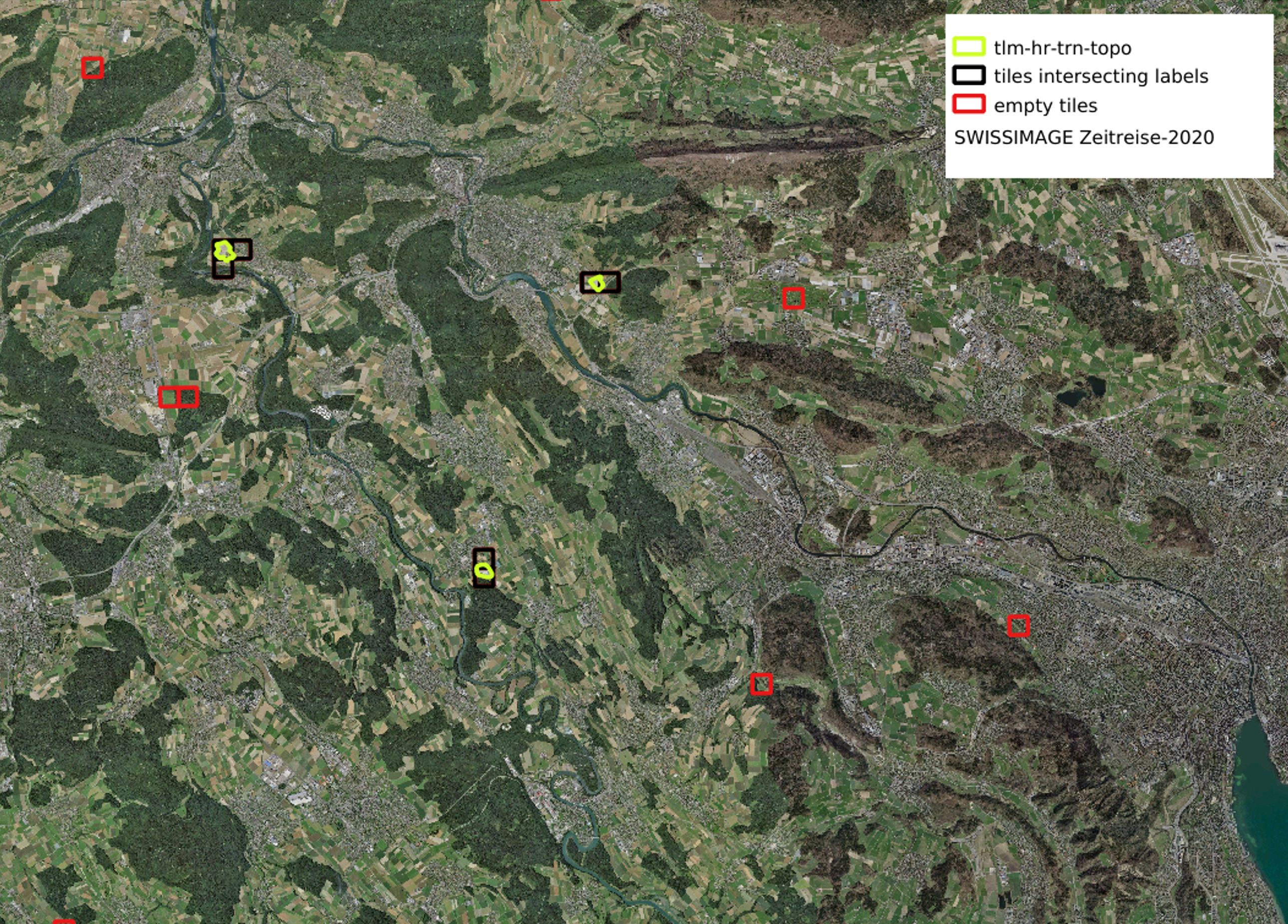
Figure A1: View of tiles intersecting (black) labels (yellow) and randomly selected empty tiles (red) in Switzerland. This case correspond to the addition of 35% empty tiles.

Figure A1 reveals that adding empty tiles to the dataset does not significantly influence the metrics values. The number of TP, FP, and FN do not show significant variation. However, when performing an inference detection test on a subset of tiles (2000) for an AOI, it appears that the number of raw detections (unfiltered) is reduced as the number of empty tiles increases. However, visual inspection of the final detection after applying filters does not show significant improvement compared to a model trained without adding empty tiles.

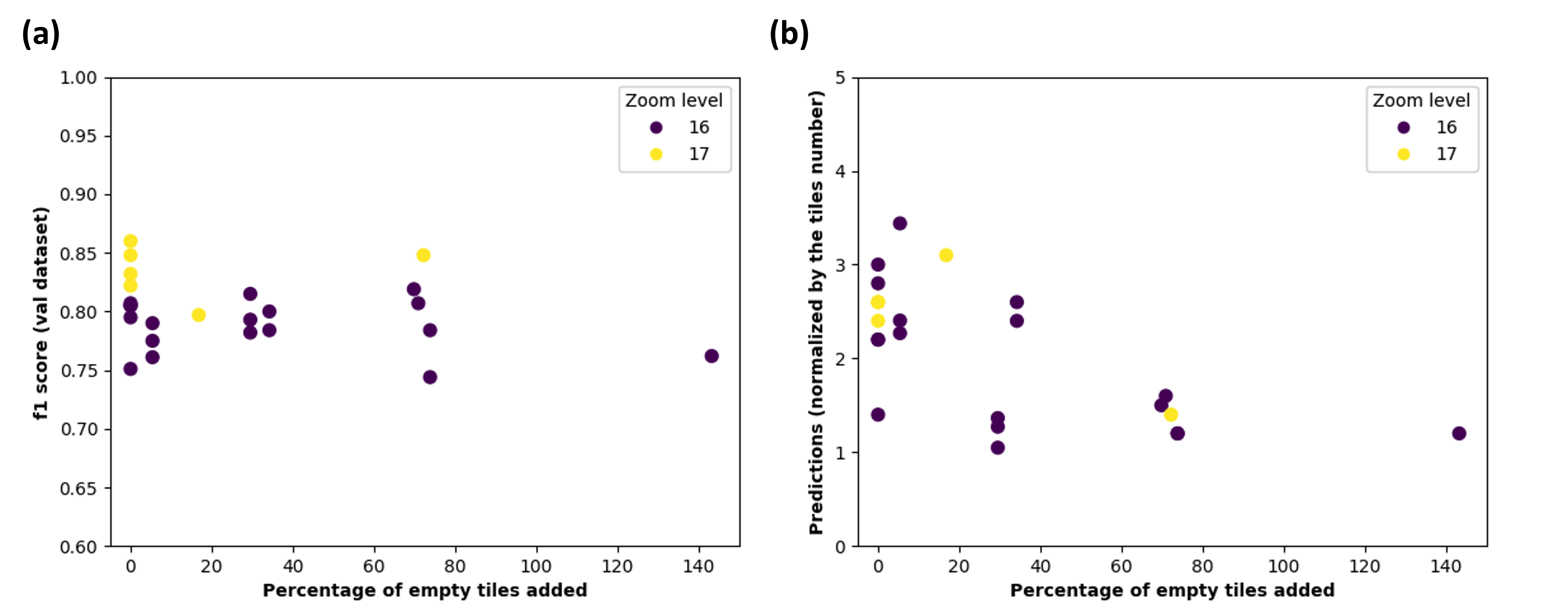
Figure A1: Influence of the addition of empty tiles (relative to the number of tiles intersecting labels) on trained performance for zoom levels 16 and 17 with (a) the F1-score as a function of the percentage of added empty tiles and (b) the normalised (by the number of tiles sampled = 2000) number of detection as a function of added empty tiles. Empty tiles have been added to only the train dataset for the 5% and 30% cases and to all datasets for 9%, 35%, 70%, and 140% cases.

A considered solution to improve the results could be to specifically select tiles for which FP occurred and include them in the training dataset as empty tiles. This way, the model could be trained with relevant confounding features such as snow patches, river sandbeds, or gullies not labeled as GT.

A.2 Sensitivity of the model to the number of images per batch

During the model learning phase, the trained model is updated after each batch of samples was processed. Adding more samples, i.e. in our case images, to the batch can influence the model learning capacity. We investigated the role of adding more images per batch for a dataset with and without adding a portion of empty tiles to the learning dataset. Adding more images per batch speeds up the model learning (Table A1), and the minimum of the loss curve is reached for a smaller number of iterations.

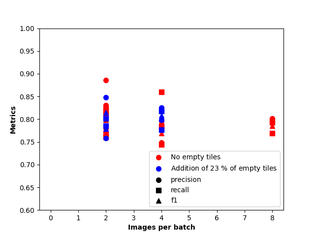
Figure A2: Metrics (precision, recall and f1-score) evolution with the number of images per batch during the model training. Results have been obtained on a dataset without empty tiles addition (red) and with the addition of 23% of empty tiles to the training dataset.

Figure A2 reveals that the metrics values remain in a range of constant values while adding extra images to the batch in all cases (with or without empty tiles). A potential effect of adding more images to the batch is the reduction of the metrics variability between replicates of trained models as the range of metrics values is smaller for 8 images per batch than 2 images per batch. However, this observation has to be taken carefully as fewer replicates have been performed with 8 images per batch than for 2 or 4 images per batch. Further investigation would provide stronger insights on this effect.

A.3 Evaluation of trained models

Table A1 sumup metrics value obtained for all the configuration tested for the project.

zoom level	model	empty tiles (%)	image per batch	optimum iteration	precision	recall	f1
15	replicate 1	0	2	1000	0.727	0.810	0.766
16	replicate 1	0	2	2000	0.842	0.793	0.817
16	replicate 2	0	2	2000	0.767	0.760	0.763
16	replicate 3	0	2	3000	0.831	0.810	0.820
16	replicate 4	0	2	2000	0.886	0.769	0.826
16	replicate 5	0	2	2000	0.780	0.818	0.798
16	replicate 6	0	2	3000	0.781	0.826	0.803
16	replicate 7	0	4	1000	0.748	0.860	0.800
16	replicate 8	0	4	1000	0.779	0.785	0.782
16	replicate 9	0	8	1500	0.800	0.793	0.797
16	replicate 10	0	4	1000	0.796	0.744	0.769
16	replicate 11	0	8	1000	0.802	0.769	0.785
16	ET-250_allDS_1	34.2	2	2000	0.723	0.770	0.746
16	ET-250_allDS_2	34.2	2	3000	0.748	0.803	0.775
16	ET-1000_allDS_1	73.8	2	6000	0.782	0.815	0.798
16	ET-1000_allDS_2	69.8	2	6000	0.786	0.767	0.776
16	ET-1000_allDS_3	70.9	2	6000	0.777	0.810	0.793
16	ET-1000_allDS_4	73.8	2	6000	0.768	0.807	0.787
16	ET-2000_allDS_1	143.2	2	6000	0.761	0.748	0.754
16	ET-80_trnDS_1	5.4	2	2000	0.814	0.793	0.803
16	ET-80_trnDS_2	5.4	2	2000	0.835	0.752	0.791
16	ET-80_trnDS_3	5.4	2	2000	0.764	0.802	0.782
16	ET-400_trnDS_1	29.5	2	6000	0.817	0.777	0.797
16	ET-400_trnDS_2	29.5	2	5000	0.848	0.785	0.815
16	ET-400_trnDS_3	29.5	2	4000	0.758	0.802	0.779
16	ET-400_trnDS_4	29.5	4	2000	0.798	0.818	0.808
16	ET-400_trnDS_5	29.5	4	1000	0.825	0.777	0.800
16	ET-1000_trnDS_1	0	2	4000	0.758	0.802	0.779
17	replicate 1	0	2	5000	0.819	0.853	0.835
17	replicate 1	0	2	5000	0.803	0.891	0.845
17	replicate 1	0	2	5000	0.872	0.813	0.841
17	ET-250_allDS_1	16.8	2	3000	0.801	0.794	0.797
17	ET-1000_allDS_1	72.2	2	7000	0.743	0.765	0.754
18	replicate 1	0	2	10000	0.864	0.855	0.859

Table A1: Metrics value computed for the validation dataset for all the trained models with the 2020 SWISSIMAGE Journey mosaic at zoom level 16.

---

1. Victor Maus, Stefan Giljum, Jakob Gutschlhofer, Dieison M. Da Silva, Michael Probst, Sidnei L. B. Gass, Sebastian Luckeneder, Mirko Lieber, and Ian McCallum. A global-scale data set of mining areas. Scientific Data, 7(1):289, September 2020. URL: https://www.nature.com/articles/s41597-020-00624-w, doi:10.1038/s41597-020-00624-w. ↩↩↩↩↩

2. Vicenç Carabassa, Pau Montero, Marc Crespo, Joan-Cristian Padró, Xavier Pons, Jaume Balagué, Lluís Brotons, and Josep Maria Alcañiz. Unmanned aerial system protocol for quarry restoration and mineral extraction monitoring. Journal of Environmental Management, 270:110717, September 2020. URL: https://linkinghub.elsevier.com/retrieve/pii/S0301479720306496, doi:10.1016/j.jenvman.2020.110717. ↩↩↩↩

3. Chunsheng Wang, Lili Chang, Lingran Zhao, and Ruiqing Niu. Automatic Identification and Dynamic Monitoring of Open-Pit Mines Based on Improved Mask R-CNN and Transfer Learning. Remote Sensing, 12(21):3474, January 2020. URL: https://www.mdpi.com/2072-4292/12/21/3474, doi:10.3390/rs12213474. ↩↩↩↩

4. Haoteng Zhao, Yong Ma, Fu Chen, Jianbo Liu, Liyuan Jiang, Wutao Yao, and Jin Yang. Monitoring Quarry Area with Landsat Long Time-Series for Socioeconomic Study. Remote Sensing, 10(4):517, April 2018. URL: https://www.mdpi.com/2072-4292/10/4/517, doi:10.3390/rs10040517. ↩↩

5. Valentin Tertius Bickel and Andrea Manconi. Decadal Surface Changes and Displacements in Switzerland. Journal of Geovisualization and Spatial Analysis, 6(2):24, December 2022. URL: https://link.springer.com/10.1007/s41651-022-00119-9, doi:10.1007/s41651-022-00119-9. ↩↩

6. George P. Petropoulos, Panagiotis Partsinevelos, and Zinovia Mitraka. Change detection of surface mining activity and reclamation based on a machine learning approach of multi-temporal Landsat TM imagery. Geocarto International, 28(4):323–342, July 2013. URL: http://www.tandfonline.com/doi/abs/10.1080/10106049.2012.706648, doi:10.1080/10106049.2012.706648. ↩

7. Huriel Reichel and Nils Hamel. Automatic Detection of Quarries and the Lithology below them in Switzerland. 2022. URL: file:///C:/Users/Clemence/Documents/STDL/Projects/proj-quarries/01_Documentation/Bibliography/Automatic%20Detection%20of%20Quarries%20and%20the%20Lithology%20below%20them%20in%20Switzerland%20-%20Swiss%20Territorial%20Data%20Lab.htm. ↩↩↩↩

8. Yuxin Wu, Alexander Kirillov, Francisco Massa, Wan-Yen Lo, and Ross Girshick. Detectron2. 2019. URL: https://github.com/facebookresearch/detectron2. ↩

9. Kaiming He, Georgia Gkioxari, Piotr Dollár, and Ross Girshick. Mask R-CNN. January 2018. arXiv:1703.06870 [cs]. URL: http://arxiv.org/abs/1703.06870, doi:10.48550/arXiv.1703.06870. ↩