Dieback of beech trees: methodology for determining the health state of beech trees from airborne images and LiDAR point clouds

Clotilde Marmy (ExoLabs) - Gwenaëlle Salamin (ExoLabs) - Alessandro Cerioni (Canton of Geneva) - Roxane Pott (swisstopo)

Proposed by the Canton of Jura - PROJ-HETRES
October 2022 to August 2023 - Published on November 13, 2023

All scripts are available on GitHub.

Abstract: Beech trees are sensitive to drought and repeated episodes can cause dieback. This issue affects the Jura forests requiring the development of new tools for forest management. In this project, descriptors for the health state of beech trees were derived from LiDAR point clouds, airborne images and satellite images to train a random forest predicting the health state per tree in a study area (5 km²) in Ajoie. A map with three classes was produced: healthy, unhealthy, dead. Metrics computed on the test dataset revealed that the model trained with all the descriptors has an overall accuracy up to 0.79, as well as the model trained only with descriptors derived from airborne imagery. When all the descriptors are used, the yearly difference of NDVI between 2018 and 2019, the standard deviation of the blue band, the mean of the NIR band, the mean of the NDVI, the standard deviation of the canopy cover and the LiDAR reflectance appear to be important descriptors.

1. Introduction

Since the drought episode of 2018, the canton of Jura and other cantons have noticed dieback of the beech trees in their forests ¹. In the canton of Jura, this problem mainly concerns the Ajoie region, where 1000 hectares of deciduous trees are affected ². This is of concern for the productivity and management of the forest, as well as for the security of walkers. In this context, the République et Canton du Jura has contacted the Swiss Territorial Data Lab to develop a new monitoring solution based on data science, airborne images and LiDAR point clouds. The dieback symptoms are observable in the mortality of branches, the transparency of the tree crown and the leaf mass partition ³.

The vegetation health state influences the reflectance in images (airborne and satellite), which is often used as a monitoring tool, in particular under the form of vegetation indices:

• Normalized Difference Vegetation Index (NDVI), a combination of the near-infrared and red bands quantifying vegetation health;
• Vegetation Health Index (VHI), an index quantifying the decrease or increase of vegetation in comparison to a reference state.

For instance, Brun et al. studied early-wilting in Central European forests with time series of the Normalized Difference Vegetation Index (NDVI) and estimate the surface concerned by early leaf-shedding ⁴.

Another technology used to monitor forests is light detection and ranging (LiDAR) as it penetrates the canopy and gives 3D information on trees and forest structures. Several forest and tree descriptors such as the canopy cover ⁵ or the standard deviation of crown return intensity ⁶ can be derived from the LiDAR point cloud to monitor vegetation health state.

In ⁵, the study was conducted at tree level, whereas in ⁶ stand level was studied. To work at tree level, it is necessary to segment individual trees in the LiDAR point cloud. On complex forests, like with a dense understory near tree stems, it is challenging to get correct segments without manual corrections.

The aim of this project is to provide foresters with a map to help plan the felling of beech trees in the Ajoie's forests. To do so, we developed a combined method using LiDAR point clouds and airborne and satellite multispectral images to determine the health state of beech trees.

2. Study area

The study was conducted in two areas of interest in the Ajoie region (Fig. 1.A); one near Miécourt (Fig. 1.B), the other one near Beurnevésin (Fig. 1.C). Altogether they cover 5 km², 1.4 % of the Canton of Jura's forests ⁷.

Miécourt sub-area is west-south and south oriented, whereas Beurnevésin sub-area is rather east-south and south oriented. They are in the same altitude range (600-700 m) and are 2 km away from each other, thus near the same weather station.

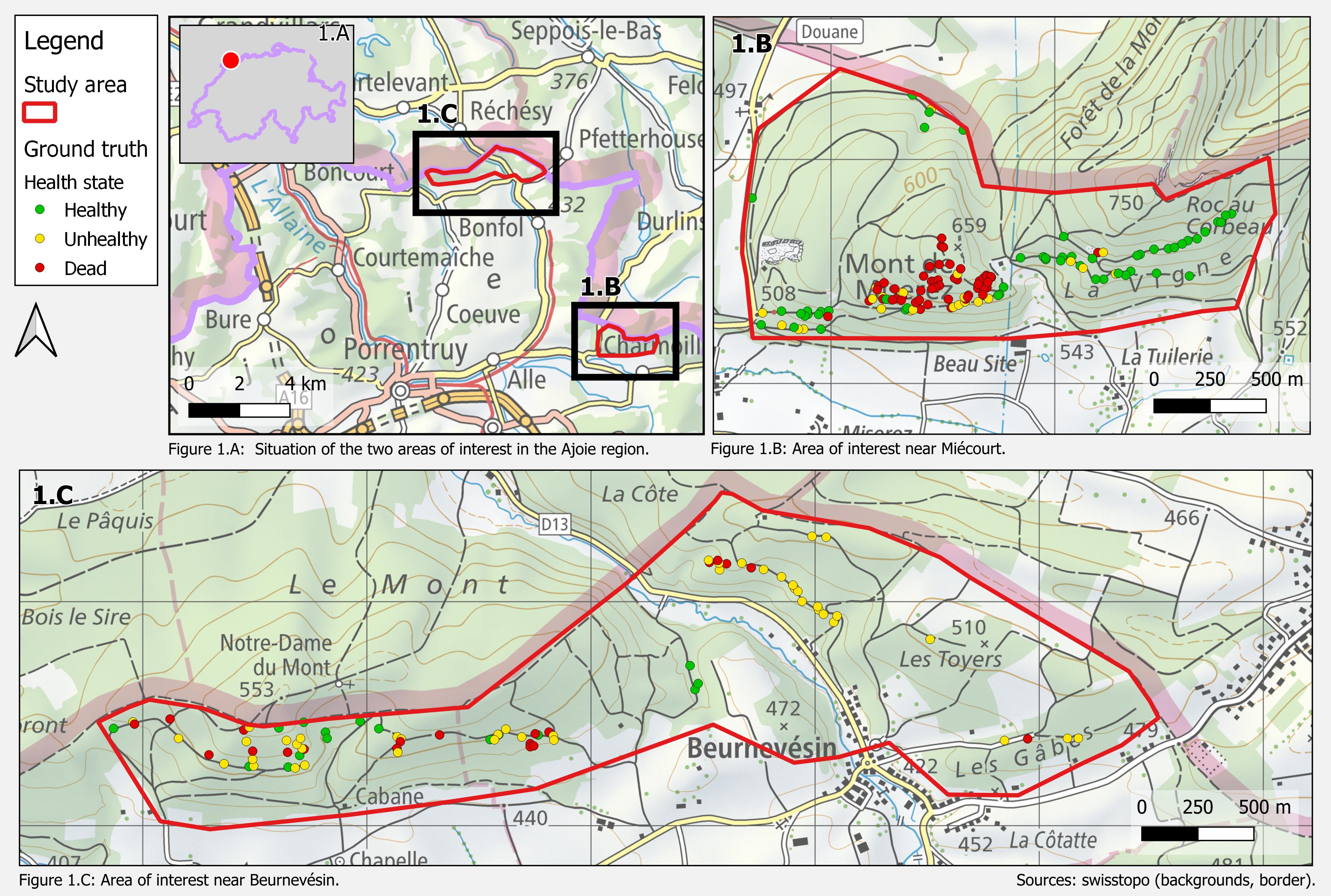
Figure 1: The study area is composed of two areas of interest.

3. Data

The project makes use of different data types: LiDAR point cloud, airborne and satellite imagery, and ground truth data. Table 1 gives an overview of the data and their characteristics. Data have been acquired in late summer 2022 to have an actual and temporally correlated information on the health state of beech trees.

Table 1: Overview of the data used in the project.

	Resolution	Acquisition time	Proprietary
LiDAR	50-100 pts/m2	08.2022	République et Canton du Jura
Airborne images	0.03 m	08.2022	République et Canton du Jura
Yearly variation of NDVI	10 m	06.2015-08.2022	Bern University of Applied Science (HAFL) and the Federal Office for Environment (BAFU)
Weekly vegetation health index	10 m	06.2015-08.2022	ExoLabs
Ground truth	- (point data)	08.-10.2022	République et Canton du Jura

3.1 LiDAR point cloud

The LiDAR dataset was acquired on the 16th of August 2023 and its point density is 50-100 pts/m². It is classified in the following classes: ground, low vegetation (2-10m), middle vegetation (10-20m) and high vegetation (20 m and above). It was delivered in the LAS format and had reflectance values ⁸ in the intensity storage field.

3.2 Airborne images

The airborne images have a ground resolution of 3 cm and were acquired simultaneously to the LiDAR dataset. The camera captured the RGB bands, as well as the near infrared (NIR) one. The acquisition of images with a lot of overlap and oblique views allowed the production of a true orthoimage for a perfect match with the LiDAR point cloud and the data of the ground truth.

3.3 Satellite images

The Sentinel-2 mission from the European Space Agency is passing every 6 days over Switzerland and allows free temporal monitoring at a 10 m resolution. The archives are available back to the beginning of beech tree dieback in 2018.

3.3.1 Yearly variation of NDVI

The Bern University of Applied Science (HAFL) and the Federal Office for Environment (BAFU) have developed Web Services for vegetation monitoring derived from Sentinel-2 images. For this project, the yearly variation of NDVI ⁹ between two successive years is used. It measures the decrease in vegetation activity between August of one year (e.g. 2018) and June of the following year (e.g. 2019). The decrease is derived from rasters made of maximum values of the NDVI in June, July or August. The data are downloaded from the WCS service which delivers "row" indices: the NDVI values are not cut for a minimal threshold.

3.3.2 VHI

The Vegetation Health Index (VHI) was generated by ETHZ, WSL and ExoLab within the SILVA project ¹⁰ which proposes several indices for forest monitoring. VHI from 2016 to 2022 is used. It is computed mainly out of Sentinel-2 images, but also out of images from other satellite missions, in order to have data to obtain a weekly index with no time gap.

3.4 Ground truth

The ground truth was collected between August and October 2022 by foresters. They assessed the health of the beech trees based on four criteria ³:

1. mortality of branches;
2. transparency of the tree crown;
3. leaf mass partition;
4. trunk condition and other health aspects.

In addition, each tree was associated with its coordinates and pictures as illustrated in Figure 1 and Figure 2 respectively. The forester surveyed: 75 healthy, 77 unhealthy and 56 dead trees.

Tree locations were first identified in the field with a GPS-enabled tablet on which the 2022 SWISSIMAGE mosaic was displayed. Afterwards, the tree locations were precisely adjusted on the trunk locations by visually locating the corresponding stems in the LiDAR point cloud with the help of the pictures taken in the field. The location and health status of a further 18 beech trees were added in July 2023. These 226 beeches - under which are 76 healthy, 77 affected and 73 dead trees - surveyed at the two dates are defined as the ground truth for this project.

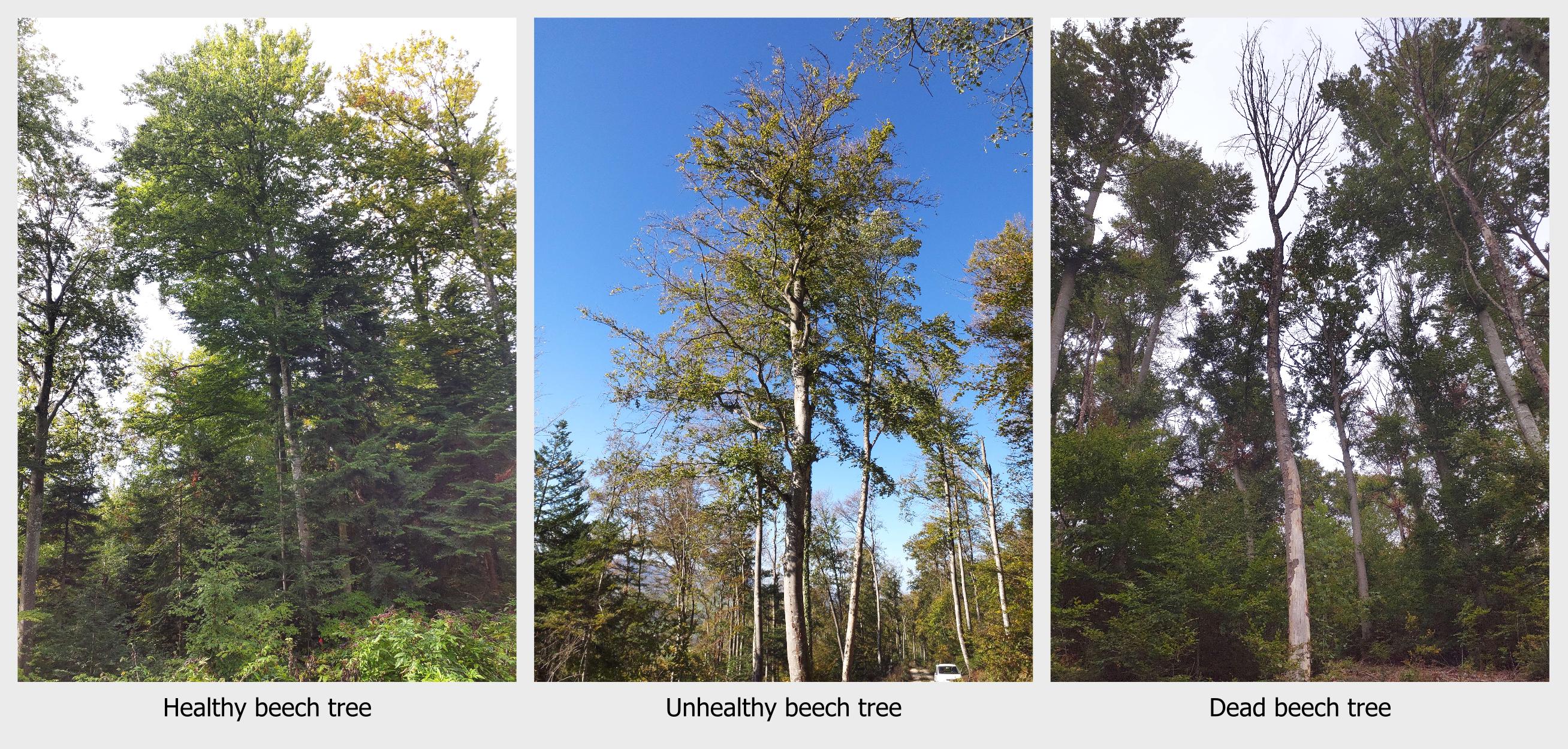
Figure 2: Examples of the three health states: left, a healthy tree with a dense green tree crown; center, an unhealthy tree with dead twigs and a scarce foliage; right, a dead tree completely dry.

4. Method

The method developed is based on the processing of LiDAR point clouds and of airborne images. Ready-made vegetation indices derived from satellite imagery were also used. First, a segmentation of the trees in the LiDAR point cloud was carried out using the Digital-Forestry-Toolbox (DFT) ¹¹. Then, descriptors for the health state of the beech trees were derived from each dataset. Boxplots and corresponding t-test are computed to evaluate the ability of descriptors to differentiate the three health states. A t-test value below 0.01 indicates that there is a significant difference between the means of two classes. Finally, the descriptors were used jointly with the ground truth to train a random forest (RF) algorithm, before inferring for the study area.

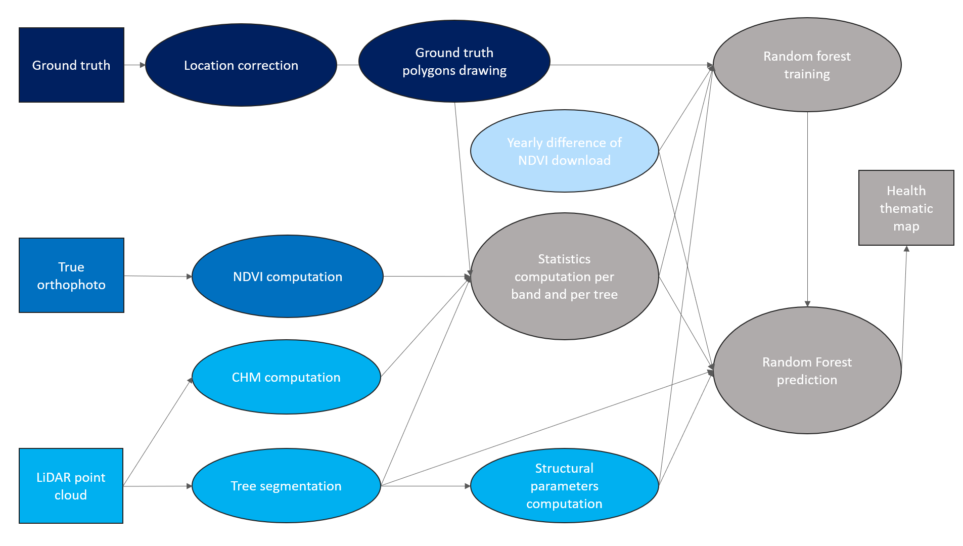
Figure 3: Overview of the methodology, which processes the data into health descriptors for beech trees, before training and evaluating a random forest.

4.1 LiDAR processing

At the beginning of LiDAR processing, exploration of the data motivated the segmentation and descriptors computation.

4.1.2 Data exploration

In order to get an understanding of the available information at the tree level, we manually segmented three healthy, five unhealthy and three dead trees. More unhealthy trees have been segmented to better represent dieback symptoms. Vertical slices of each tree were rotary extracted, providing visual information on the health state.

4.1.3 Segmentation

To be able to describe the health state of each tree, segmentation of the forest was performed using the DFT. Parameters have been tuned to find an appropriate segmentation. Two strategies for peak isolation were tested on the canopy height model (CHM):

1. Maxima smoothing: a height difference is set below which all local maxima are suppressed.
2. Local maxima within search radius: the size of the dilation window for identification of maxima is dependent on the height.

Each peak isolation method was tested on a range of parameters and on different cell resolutions for the CHM computation. The detailed plan of the simulation is given in Appendix 1. The minimum tree height was set to 10 m. For computation time reasons, only 3 LiDAR tiles with 55 ground truth (GT) trees located on them were processed.

To find the best segmentation, the locations of the GT trees were compared to the location of the segment peaks. GT trees with a segmented peak less than 4 m away were considered as True Positive (TP). The best segmentation was the one with the most TP.

4.1.4 Structural descriptors

An alternative to the segmentation is to change of paradigm and perform the analyses at the stand level. Meng et al. ⁶ derived structural descriptors for acacia dieback at the stand level based on LiDAR point cloud. By adapting their method to the present case, the following descriptors were derived from the LiDAR point cloud using the LidR library from R ¹²:

1. Canopy maximal height.
2. Scale and shape parameters of the Weibull density function fitted for the point distribution along the height.
3. Coefficient of variation of leaf area density (cvLAD) describing the distribution of the vertical structure of photosynthetic tissue along the height.
4. Vertical Complexity Index (VCI): Entropy measure of the vertical distribution of vegetation.
5. Standard deviation of the canopy height model (sdCHM), reflects canopy height variations.
6. Canopy cover (CC) and standard deviation (sdCC), reflects foliage density and coverage.
7. Above ground biomass height (AGH), reflects the understory height until 10 m.

Descriptors 1 to 6 are directly overtaken from Meng et al. All the descriptors were first computed for three grid resolutions: 10 m, 5 m and 2.5 m.
In a second time, the DFT segments were considered as an adaptive grid around the trees, with the assumption that it is still more natural than a regular grid. Then, structural descriptors for vertical points distribution (descriptors 1 to 4) were computed on each segment, whereas descriptors for horizontal points distribution (descriptors 5 to 7) have been processed for 2.5 m grid. A weight was applied to the value of the latter descriptors according to the area of grid cells included in the footprint of the segments.

Furthermore, LiDAR reflectance mean and standard deviation (sd) were computed for the segment crowns to differentiate them by their reflectance.

4.2 Image processing

For the image processing, an initial step was to compute the normalized difference vegetation index (NDVI) for each raster image. The normalized difference vegetation index (NDVI) is an index commonly used for the estimation of the health state of vegetation ⁵¹³¹⁴.

\[\begin{align} \ NDVI = {NIR-R \over NIR+R} \ \end{align}\]

where NIR and R are the value of the pixel in the near-infrared and red band respectively.

To uncover potential distinctive features between the classes, boxplots and principal component analysis were used on the images four bands (RGB-NIR) and the NDVI.

Firstly, we tested if the brute pixel values allowed the distinction between classes at a pixel level. This method avoids the pit of the forest segmentation into trees.
Secondly, we tested the same method, but with some low-pass filter to reduce the noise in the data.
Thirdly, we tried to find distinct statistical features at the tree level. This approach allows decreasing the noise that can be present in high-resolution information. However, it necessitates having a reasonably good segmentation of the trees.
Finally, color filtering and edge detection were tested in order to highlight and extract the linear structure of the branches.

For each treatment, it is possible to do it with or without a mask on the tree height. As only trees between 20 m and 40 m tall are affected by dieback, a mask based on the Canopy Height Model (CHM) raster derived from the LiDAR point cloud was tested.

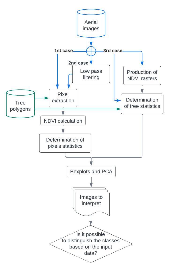
Figure 4: Overview of different possible data treatments for the the statistical analysis.

4.2.1 Statistical tests on the original and filtered pixels

The statistical tests were performed on the original and filtered pixels.

Two low pass filters were tested:

• Gaussian with a sigma of 5;
• Bilinear downsampling with scale factors of 1/3, 1/5 and 1/17, corresponding to resolutions of 9, 15 and 50 cm.

In the original and the filtered cases, the pixels for each GT tree were extracted from the images and sorted by class. Then, the corresponding NDVI is computed. Each pixel has 5 attributes corresponding to its value on the four bands (R, G, B, NIR) and its NDVI.
First, the per-class boxplots of the attributes were executed to see if the distinction between classes was possible on one or several bands or on the NDVI.
Then, the principal component analysis (PCA) was computed on the same values to see if their linear combination allowed the distinction of the classes.

4.2.2. Statistical tests at the tree level

For the tests at the tree level, the GT trees were segmented by hand. For each tree, the statistics of the pixels were calculated over its polygon, on each band and for the NDVI. Then, the results were sorted by class.
Each tree has five attributes per band or index corresponding to the statistics of its pixels: minimum (min), maximum (max), mean, median and standard deviation (std).

Like with the pixels, the per-class boxplots of the attributes were executed to see if the distinction between classes was possible. Then, the PCA was computed.

4.2.3 Extraction of branches

One of the beneficiaries noted that the branches are clearly visible on the RGB images. Therefore, it may be possible to isolate them with color filtering based on the RGB bands.
We calibrated an RGB filter through trial and error to produce a binary mask indicating the location of the branches. A sieve filter was used to reduce the noise due to the lighter parts of the foliage. Then, a binary dilation was performed on the mask to highlight the results. Otherwise, they would be too thin to be visible at a 1:5'000 scale.
A mask based on the CHM is integrated to the results to limit the influence of the ground.

The branches have a characteristic linear structure. In addition, the branches of dead trees tend to be very light line on the dark forest ground and understory. Therefore, we thought that we may detect the dead branches thanks to edge detection. We used the canny edge detector and tested the python functions of the libraries openCV and skimage.

4.3 Satellite-based indices

The yearly variation of NDVI and the VHI were used to take account of historical variations of NDVI from 2015 to 2022. For the VHI, the mean for each year is computed over the months considered for the yearly variation of NDVI.

The pertinence of using these indices was explored: the values for each tree in the ground truth were extracted and observed in boxplots per health class in 2022 per year pair over the time span from 2015 to 2022.

4.4 Random Forest

In R ¹², the caret and randomForest packages were used to train the random forest and make predictions. First, the ground truth was split into the training and the test datasets, with each class being split 70 % into the training set and 30 % into the test set. Health classes with not enough samples were completed with copies. Optimization of the RF was performed on the number of trees to develop and on the number of randomly sampled descriptors to test at each split. In addition, 5-fold cross-validation was used to ensure the use of different parts of the dataset. The search parameter space was from 100 to 1000 decision trees and from 4 to 10 descriptors as the default value is the square root of all descriptors, i.e. 7. RF was assessed using a custom metric, which is an adaptation of the false positive rate for the healthy class. It minimizes the amount of false healthy detections and of dead trees predicted as unhealthy (false unhealthy). It is called custom false positive rate (cFPR) in the text. It was preferred to have a model with more unhealthy predictions to control on the field, than missing unhealthy or dead trees. The cFPR goes from 0 (best) to 1 (worse).

Table 2: Confusion matrix for the three health classes.

		Ground truth
		Healthy	Unhealthy	Dead
Prediction	Healthy	A	B	C
	Unhealthy	D	E	F
	Dead	G	H	I

According to the confusion matrix in Table 2, the cFPR is computed as follows:

\[\begin{align} \ cFPR = {(𝐵+𝐶+𝐹)\over(𝐵+𝐶+𝐸+𝐹+𝐻+𝐼)}. \ \end{align}\]

In addition, the overall accuracy (OA), i.e. the ratio of correct predictions over all the predictions, and the sensitivity, which is, per class, the number of correct predictions divided by the number of samples from that class, are used.

An ablation study was performed on descriptors to assess the contribution of the different data sources to the final performance. An “important” descriptor is having a strong influence on the increase in prediction errors in the case of random reallocation of the descriptor values in the training set.

After the optimization, predictions for each DFT segments were computed using the best model according to the cFPR. The inferences were delivered as a thematic map with colors indicating the health state and hue indicating the fraction of decision trees in the RF having voted for the class (vote fraction). The purpose is to give a confidence information, with high vote fraction indicating robust predictions.

Furthermore, the ground truth was evaluated for quantity and quality by two means:

• Removal of samples and its impact on the metric evaluation
• Splitting the training set into training subsets to evaluate on the original test set.

Finally, after having developed the descriptors and the routine on high-quality data, we downgraded them to have resolutions similar to the ones of the swisstopo products (LiDAR: 20 pt/m², orthoimage: 10 cm) and performed again the optimization and prediction steps. Indeed, the data acquisition was especially commissioned for this project and only covers the study area. If in the future the method should be extended, one would like to test if a lower resolution as the one of the standard national-wide product SWISSIMAGE could be sufficient.

5 Results and discussion

In this section, the results obtained during the processing of each data source into descriptors are presented and discussed, followed by a section on the random forest results.

5.1 LiDAR processing

For the LiDAR data, the reader will first discover the aspect of beech trees in the LiDAR point cloud according to their health state as studied in the data exploration. Then, the segmentation results and the obtained LiDAR-based descriptors will be presented.

5.1.2 Data exploration for 11 beech trees

The vertical slices of 11 beech trees provided visual information on health state: branch shape, clearer horizontal and vertical point distribution. In Figure 5, one can appreciate the information shown by these vertical slices. The linear structure of the dead branches, the denser foliage of the healthy tree and the already smaller tree crown of the dead tree are well recognizable.

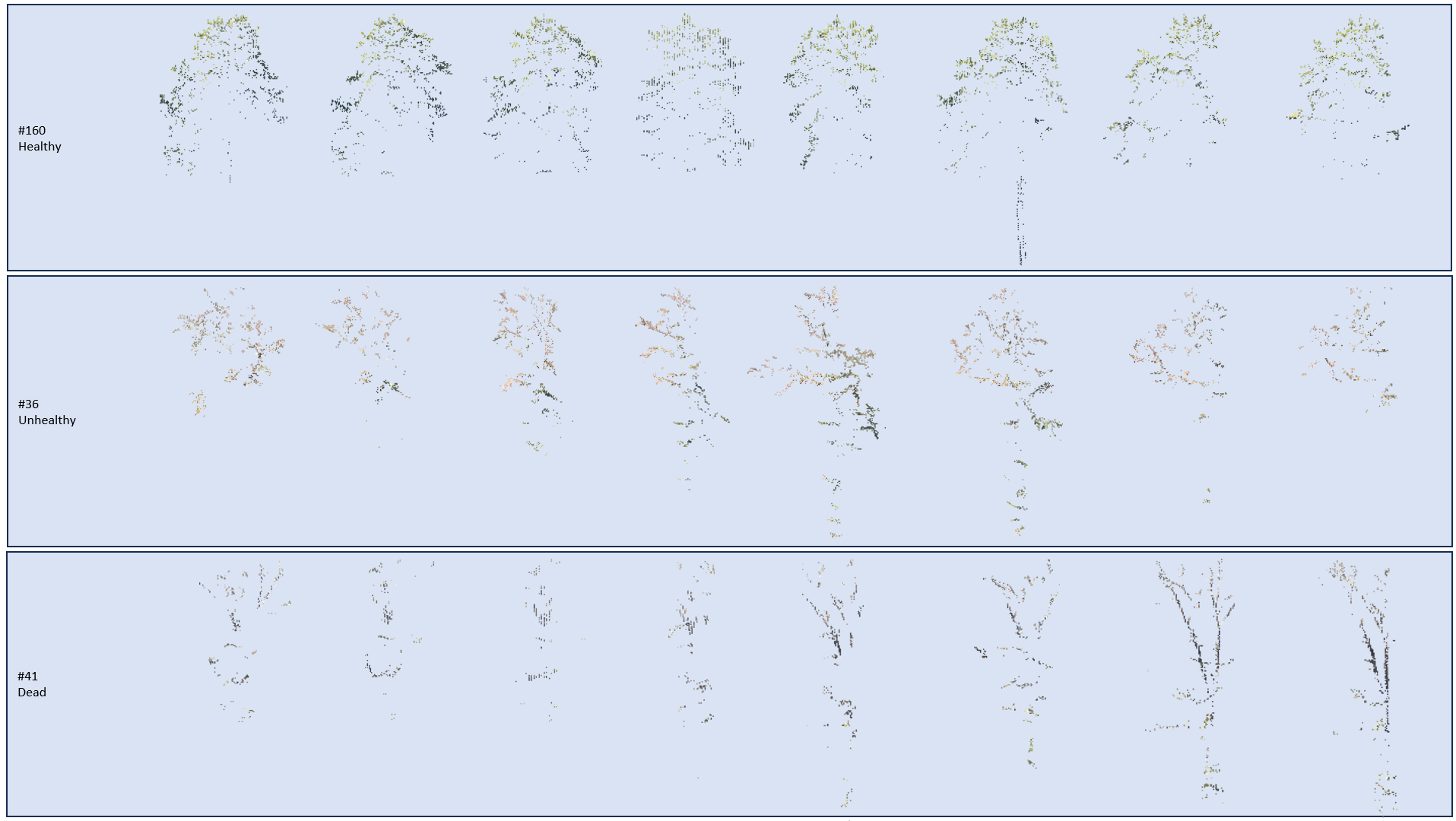
Figure 5: Slices for three trees with different health state. Vertical slices of each tree were rotary extracted, providing visual information on the health state. Dead twigs and density of foliage are particularly distinctive.

Some deep learning image classifier could treat LiDAR point cloud slices as artificial images and learn from them before classifying any arbitrary slice from the LiDAR point cloud. However, the subject is not adapted to transfer learning because 200 samples are not enough to train a model to classify three new classes, especially via images without resemblance to datasets used to pre-train deep learning models.

5.1.3 Segmentation

Since the tree health classes were visually recognizable for the 11 trees, it was very interesting to individuate each tree in the LiDAR point cloud.

After having searched for optimal parameters in the DFT, the best realization of each peak isolation method either slightly oversegmented or slightly undersegmented the forest. The forest has a complex structure with dominant and co-dominant trees, and with understory. A simple yet frequent example is the situation of a small pine growing in the shadow of a beech tree. It is difficult for an algorithm to differentiate between the points belonging to the pine and those belonging to the beech. Complex tree crowns (not spheric, with two maxima) especially lead to oversegmentation.

As best segmentation, the smoothing of maxima on a 0.5 m resolution CHM was identified. Out of 55 GT trees, 52 were within a 4 m distance from the centroid of a segment. The total number of segments is 7347. This corresponds to 272 trees/ha. Report of a forest inventory in the Jura forest between 2003 and 2005 indicated a density of 286 trees/ha in high forest ⁷. Since the ground truth is only made of point coordinates, it is difficult to assess quantitatively the correctness of the segments, i.e. the attribution of each point to the right segment. Therefore, the work at the tree level is only approximate.

5.1.4 Structural descriptors

Nevertheless, the structural descriptors for each tree were computed from the segmented LiDAR point cloud. The t-test between health classes for each descriptor at each resolution (10 m, 5 m, 2.5 m and per-tree grid) are given in Appendices 2, 3, 4 and 5. The number of significant descriptors per resolution is indicated to understand better the effect on the RF:

• at 10 m: 13
• at 5 m: 17
• at 2.5 m: 18
• per tree: 15

The simulations at 5 m and at 2.5 m seemed a priori the most promising. In both constellations, t-tests indicated a significant different distribution for:

• maximal height, between the three health states,
• sdCHM, between the three health states,
• cvLAD, healthy trees against the others,
• mean reflectance, healthy trees against the others,
• VCI, healthy trees against unhealthy trees,
• canopy cover, healthy trees against dead trees,
• standard deviation of the reflectance, dead trees against the others,
• sdCC, dead trees against the others.

The maximal height and the sdCHM appear to be the most suited descriptors to separate the three health states. The other descriptors are differentiating healthy trees from the others or dead trees from the others. From the 11 LiDAR-based descriptors, 8 are at least significant for the comparison between two classes.

5.2 Image processing

Boxplots and PCA are given to illustrate the results of the image processing exploration. As the masking of pixels below and above the affected height made no difference in the interpretation of the results, they are presented here with the height mask.

5.2.1 Boxplots and PCA over the pixel values of the original images

When the pixel values of the original images per health class are compared in boxplots (ex. Fig. 6), the sole brute value of the pixel is not enough to clearly distinguish between classes.

Figure 6: Boxplots of the unfiltered pixel values on the different bands and the NDVI index by health class.

The PCA in Figure 7 shows that it is not possible to distinguish the groups based on a linear combination of the brute pixel values of the band and NDVI.

Figure 7: Distribution of the pixels in the space of the principal components based on the pixel values on the different branches and the NDVI.

5.2.2 Boxplots and PCA over the pixel values of the filtered images

A better separation of the different classes is noticeable after the application of a Gaussian filter. The most promising band is the NIR one for a separation of the healthy and dead classes. On the NDVI, the distinction between those two classes should also be possible as illustrated in Figure 8. In all cases, there is no possible distinction between the healthy and unhealthy classes.
The separation between the healthy and dead trees on the NIR band would be around 130 and the slight overlap on the NDVI band is between approx. 0.04 and approx. 0.07.

Figure 8: Boxplots of the pixel values on the different bands and the NDVI by health class after a Gaussian filter with sigma=5.

As for the brute pixels, the overlap between the different classes is still very present in the PCA (Fig. 9).

Figure 9: Distribution of the pixels in the space of the principal components based on the pixel values on the different branches and the NDVI after a Gaussian filter with sigma=5.

The boxplots produced on the resampled images (Figure 10) give similar results to the ones with the Gaussian filter. The healthy and dead classes are separated on the NIR band around 130. The unhealthy class stays similar to the healthy one.

Figure 10: Boxplots of the pixel values on the different bands and the NDVI by health class after a downsampling filter with a factor 1/3.

According to the PCA in Figure 11, it seems indeed not possible to distinguish between the classes only with the information presented in this section.

Figure 11: Distribution of the pixels in the space of the principal components based on the pixel values on the different branches and the NDVI after a downsampling filter with a factor 1/3.

When the factor for the resampling is decreased, i.e. when the resulting resolution increases, the separation on the NIR band becomes stronger. With a factor of 1/17, the healthy and dead classes on the NDVI are almost entirely separated around the value of 0.04.

5.2.3 Boxplots and PCA over the tree statistics

As an example for the per-tree statistics, the boxplots and PCA for the blue band are presented in Figures 12 to 14.
On the mean and on the standard deviation, healthy and dead classes are well differentiated on the blue band as visible on Figure 12. The same is observed on the mean, median, and minimum of the NDVI, as well as on the maximum, mean, and median of the NIR band. However, there is no possible differentiation on the red and green bands.

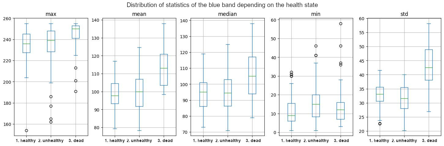
Figure 12: Boxplots of the statistics values for each tree on the blue band by health class.

In the PCA in Figure 13, the groups of the healthy and dead trees are quite well separated, mostly along the first component.

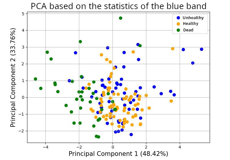
Figure 13: Distribution of the trees in the space of the principal components based on their statistical values on the blue band.

On Figure 14, the first principal component is influenced principally by the standard deviation of the blue band. The mean, the median and the max have an influence too. This is in accordance with the boxplots where the standard deviation values presented the largest gap between classes.

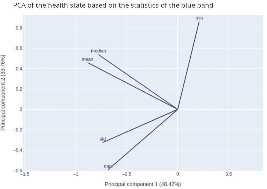
Figure 14: Influence of the statistics for the blue band on the first and second principal components.

The point clouds of the dead and healthy classes are also well separated on the PCA of the NIR band and of the NDVI. No separation is visible on the PCA of the green and red bands.

5.2.4 Extraction of branches

Finally, the extraction of dead branches was performed.

Use of an RGB filter

The result of the RGB filter is displayed in Figure 15. It is important to include the binary CHM in the visualization. Otherwise, the ground can have a significant influence on certain zones and distract from the dead trees. Some interferences can still be seen among the coniferous trees that have a similar light color as dead trees.

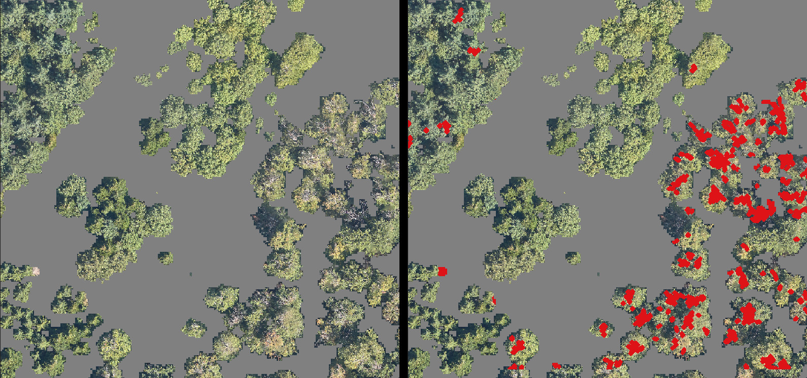
Figure 15: Results produced by the RGB filter for the detection and highlight of dead branches over a zone with coniferous, healthy deciduous and dead deciduous trees. The parts in grey are the zones masked by the filter on the height.

Use of the canny edge detector

Figure 16 presents the result for the blue band which was the most promising one. The dead branches are well captured. However, there is a lot of noise around them due to the high contrasts in some parts of the foliage. The result is not usable as is.
Using a stricter filter decreased the noise, but it also decreased the captured pixels of the branches. In addition, using a sieve filter or trying to combine the results with the ones of the RGB filter did not improve the situation.

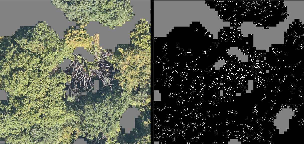
Figure 16: Test of the canny edge detector from sklearn over a dead tree by using only the blue band. The parts in grey are the zones masked by the CHM filter on the height.

The results for the other bands, RGB images or the NDVI were not usable either.

5.2.5 Discussion

The results at the tree level are the most promising ones. They are integrated into the random forest. Choosing to work at the tree-level means that all the trees must be segmented with the DFT. This adds uncertainties to the results. As explained in the dedicated section, the DFT has a tendency of over/under-segmenting the results.
The procedures at the pixel level, whether on filtered or unfiltered images, are abandoned.

For the branch detection, the results were compared with some observations on the terrain by a forest expert. He assessed the result as incorrect in several parts of the forest. Therefore, the use of dead branch detection was not integrated in the random forest.
In addition, the edge detection was maybe not the right choice for dead branches and maybe we should have taken an approach more focused on detection of straight lines or graphs. The chance of success of such methods are difficult to predict as there can be a lot of variations in the form of the dead branches.

5.3 Vegetation indices from satellite imagery

The t-test used to evaluate the ability of satellite indices to differentiate between health states are given in Appendices 6 and 7. In the following two subsections, solely the significant tested groups are mentioned for understanding the RF performance.

5.3.1 Yearly variation of NDVI

t-test on the yearly variation of NDVI indicated significance between:

• all health states in 2018-2019: 2018 was an especially dry and hot year, whereas 2019 was in the seasonal normals. The recovery in 2019 may have differed according to the health classes.
• healthy and other trees in 2016-2017 and 2019-2020: maybe healthy trees are responding diversely to environmental factors than affected trees.
• healthy and dead trees in 2021-2022: this reflects a higher increase of NDVI for the dead trees. Is the understory benefitting from clearer forest structure?

5.3.2 Vegetation Healthy Index

t-test on the VHI indicated significance between:

• dead and other trees in 2017
• healthy and dead trees in 2018
• healthy and other trees in 2019
• unhealthy and other trees in 2021
• dead and unhealthy trees in 2020 and 2022

Explanations similar to those for NDVI may partly explain the significance obtained. In any case,it is encouraging that the VHI helps to differentiate health classes thanks to different evolution through the years.

5.4 Random Forest

The results of the RF that are presented and discussed are: (1) the optimization and ablation study, (2) the ground truth analysis, (3) the predictions for the AOI and (4) the performance with downgraded data.

5.4.1 Optimization and ablation study

In Table 3, performance for VHI and yearly variation of NDVI (yvNDVI) descriptors using their value at the location of the GT trees are compared. VHI (cFPR = 0.24, OA = 0.63) performed better than the yearly variation of NDVI (cFPR = 0.39, OA = 0.5). Both groups of descriptors are mostly derived from satellite data with the same resolution (10 m). A conceptual difference is that the VHI is a deviation to a long-term reference value; whereas the yearly variation of NDVI reflects the change between two years. For the latter, values can be high or low independently of the actual health state. Example, a succession of two bad years will indicate few to no differences in NDVI.

Table 3: RF performance with satellite-based descriptors.

Descriptors	cFPR	OA
VHI	0.24	0.63
yvNDVI	0.39	0.5

Nonetheless, only the yearly variation of NDVI is used hereafter as it is available free of charge.

Regarding the LiDAR descriptors, the tested resolutions indicated that the 5 m resolution (cFPR = 0.2 and OA = 0.65) was performing the best for the cFPR, but that the per-tree descriptors had the higher OA (cFPR = 0.33, OA = 0.67). At 5 m resolution, fewer affected trees are missed, but there are more errors in the classification, so more control on the field would have to be done. The question of which grid resolution to use on the forest is a complex one, as the forest consists of trees of different sizes. Further, even if dieback affects some areas more severely than others, it's not a continuous phenomenon, and it is important to be able to clearly delimit each tree. However, a grid, as the 2.5 m one, can also hinder to capture the entirety of some trees and the performance may decrease (LiDAR, 2.5 m, OA=0.63).

Table 4: RF performance with LiDAR-based descriptors at different resolutions.

Descriptors	cFPR	OA
LiDAR, 10 m	0.3	0.6
LiDAR, 5 m	0.2	0.65
LiDAR, 2.5 m	0.28	0.63
LiDAR, per tree	0.33	0.67

Then, the 5 m resolution descriptors are kept for the rest of the analysis according to the decision of reducing missed dying trees.

The ablation study performed on the descriptor sources is summarized in Table 5.A and Table 5.B. The two tables reflect performance for two different partitions of the samples in training and test sets. Since the performance is varying form several percents, the performance is impacted by the repartition of the samples. Following those values, the best setups for each partition respectively are the full model (cFPR = 0.13, OA = 0.76) and the airborne-based model (cFPR = 0.11, OA = 0.79).

One notices that all the health classes are not predicted with the same accuracy. The airborne-based model, as described in Section 5.2.3, is less sensitive to the healthy class; whereas the satellite-based model and the LiDAR-based model is more polarized to healthy and dead classes, with low sensitivity performance in the unhealthy class.

Table 5.A: Ablation study results, partition A of the dataset.

Descriptor sources	cFPR	OA	Sensitivity healthy	Sensitivity unhealthy	Sensitivity dead
LiDAR	0.2	0.65	0.65	0.61	0.71
Airborne images	0.18	0.63	0.43	0.61	0.94
yvNDVI	0.4	0.49	0.78	0.26	0.41
LiDAR and yvNDVI	0.23	0.7	0.74	0.61	0.76
Airborne images and yvNDVI	0.15	0.73	0.65	0.7	0.88
LiDAR, airborne images and yvNDVI	0.13	0.76	0.65	0.74	0.94

Table 5.B: Ablation study results, partition B of the dataset.

Descriptor sources	cFPR	OA	Sensitivity healthy	Sensitivity unhealthy	Sensitivity dead
LiDAR	0.19	0.71	0.76	0.5	0.88
Airborne images	0.11	0.79	0.62	0.8	1
yvdNDVI	0.38	0.62	0.81	0.4	0.65
LiDAR and yvNDVI	0.27	0.74	0.86	0.5	0.88
Airborne images and yvNDVI	0.14	0.78	0.62	0.8	0.94
LiDAR, airborne images and yvNDVI	0.14	0.79	0.71	0.7	1

Even if the performance varies according to the dataset partition, the important descriptors remain quite similar between the two partitions as displayed in Figure 17.A and Figure 17.B. The yearly difference of NDVI between 2018 and 2019 (NDVI_diff_1918) is the most important descriptor; standard deviation on the blue band (b_std) and the mean on the NIR band and NDVI (nir_mean and ndvi_mean) are standing out in both cases; from the LiDAR, the standard deviation of canopy cover (sdcc) and of the LiDAR reflectance (i_sd_seg) are the most important descriptors.
The order of magnitude explains the better performance on partition B with the airborne-based model: for instance, the b_std has the magnitude of 7.6 instead of 4.6 with Partition B.

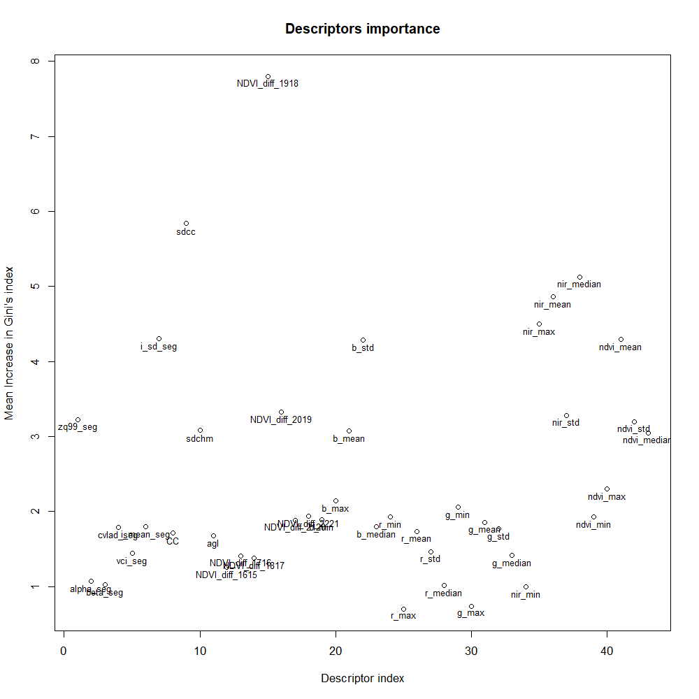
Figure 17.A: Important descriptors for the full model, dataset partition A.

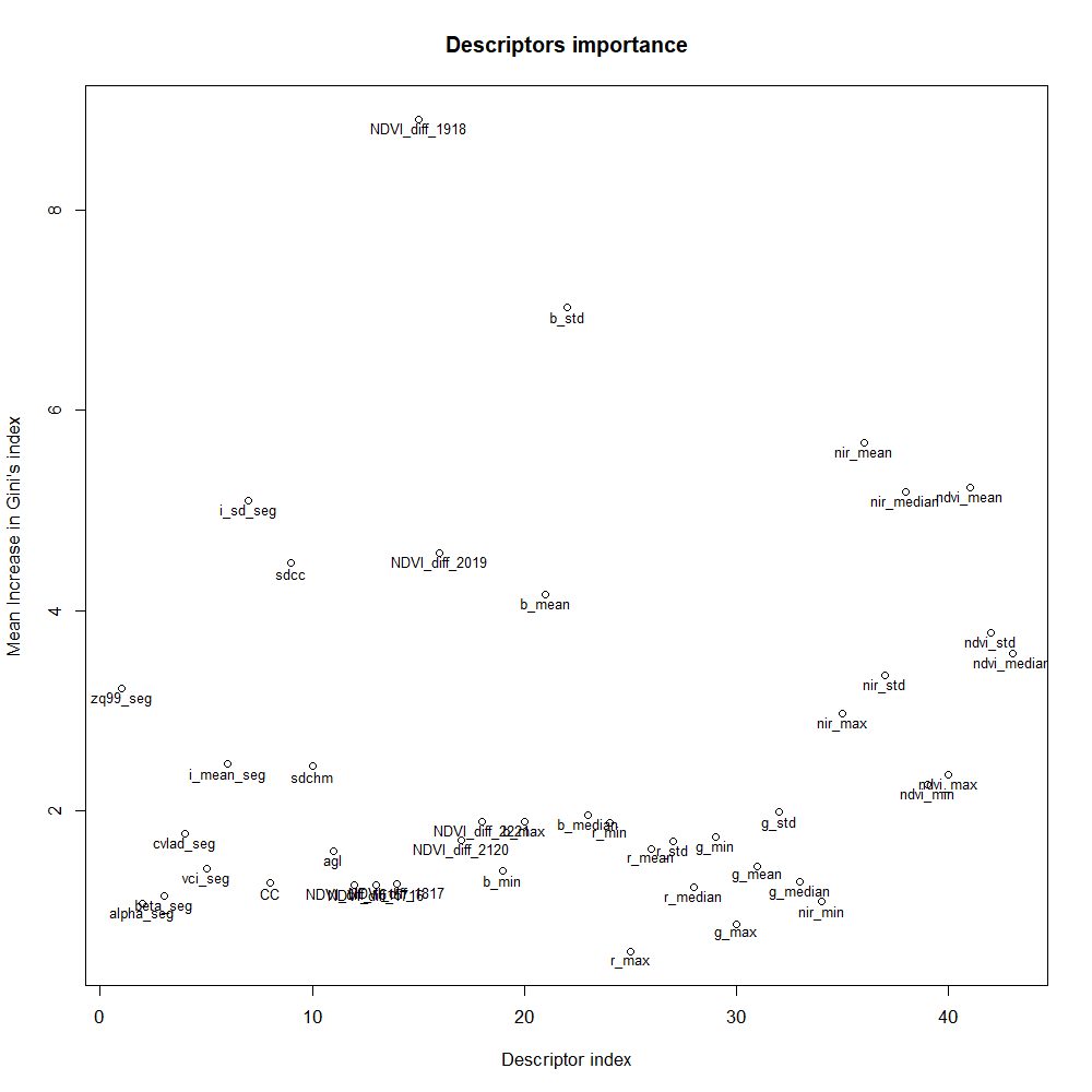
Figure 17.B: Important descriptors for the full model, dataset partition B.

The most important descriptor of the full model resulted to be the yearly variation of NDVI between 2018 and 2019. The former was a year with a dry and hot summer which has stressed beech trees and probably participated to cause forest damages ¹. This corroborates the ability of our RF method to monitor the response of trees to extreme drought events. However, the 10 m resolution of the index and the different adaptability of individual beech trees to drought may make the relationship between current health status and the index weak. This can explain that the presence of this descriptor in the full model doesn't offer better performance than the airborne-based model to predict the health state.

Both the mean on the NIR band and the standard deviation on the blue band play an important role. Statistical study in Section 5.2.3 indicated that the models might confuse healthy and unhealthy classes. On one hand, airborne imagery only sees the top of the crown and may miss useful information on hidden part. On the other hand, airborne imagery has a good ability to detect dead trees thanks to different reflectance values in NIR and blue bands.

One argument that could explain the lower performance of the model based on LiDAR-based descriptors is the difficulty to find the right scale to perform the analysis as beech trees can show a wide range of crown diameters.

5.4.2 Ground truth analysis

With progressive removal of sample individuals from the training set, impact of individual beech trees on the performance is further analyzed. The performance variation is shown in Figure 18. The performance is rather stable in the sense that the sensitivities stay in a range of values similar to the initial one up to 40 samples removed, but with each removal, a slight instability in the metrics is visible. The size of the peaks indicates variations of 1 prediction for the dead class, but up to 6 predictions for the unhealthy class and up to 7 for the healthy class. During the sample removal, some samples were always predicted correctly, whereas others were often misclassified leading to the peaks in Figure 18. With the large number of descriptors in the full model, there is no straightforward profile of outliers to identify.

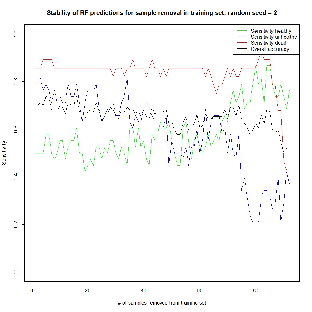
Figure 18: Evolution of the per-class sensitivity with removal of samples.

In addition, the subsampling of the training set in Table 6 shows that the OA varies only by max. 3% according to the subset used. It indicated again that the amount of ground truth allows to reach a stable OA range, but the characteristics of the samples does not allow a stable OA value. The sensitivity for the dead classes is stable, whereas sensitivity for healthy and unhealthy class are varying.

Table 6: Performance according to different random seed for the creation of the training subset.

Training set subpartition	cFPR	OA	Sensitivity healthy	Sensitivity unhealthy	Sensitivity dead
Random seed = 2	0.13	0.76	0.61	0.83	0.88
Random seed = 22	0.15	0.78	0.70	0.78	0.88
Random seed = 222	0.18	0.75	0.65	0.74	0.88
Random seed = 2222	0.13	0.76	0.65	0.78	0.88
Random seed = 22222	0.10	0.78	0.65	0.83	0.88

5.4.3 Predictions

The full model and the airborne-based-model were used to infer the health state of trees in the study area (Fig. 19). As indicated in Table 7, with the full model, 35.1 % of the segments were predicted as healthy, 53 % as unhealthy and 11.9 % as dead. With the airborne-based model, 42.6 % of the segments were predicted as healthy, 46.2 % as unhealthy and 11.2 % as dead. The two models agree on 74.3 % of the predictions. In the 25.6 % of disagreement, it is about 77.1% of disagreement between healthy and unhealthy predictions. Finally, 1.5% are critical disagreement (between healthy and dead classes).

Table 7: Percentage of health in the AOI.

Model	Healthy [%]	Unhealth [%]	Dead [%]
Full	35.1	53	11.9
Airborne-based	42.6	46.2	11.2

Control by forestry experts reported that the predictions mostly correspond to the field situation and that a weak vote fraction often corresponds to false predictions. They confirmed that the map is delivering useful information to help plan beech tree felling. The final model retained after excursion on the field is the full model.

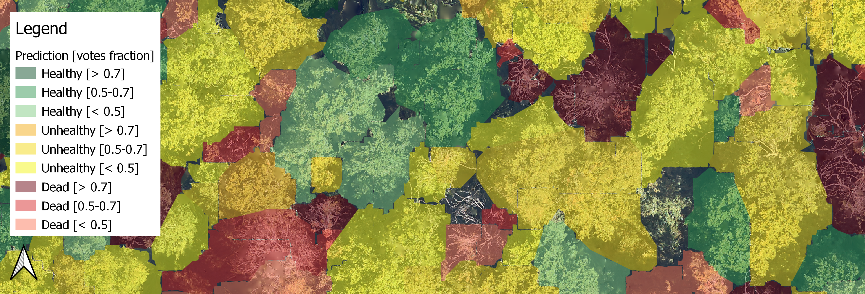
Figure 19: Extract of the predicted thematic health map. Green is for healthy, yellow for unhealthy, and red for dead trees. Hues indicate the RF fraction of votes. The predictions can be compared with the true orthophoto in the background. The polygons approximating the tree crowns correspond to the delimitation of segmented trees.

5.4.4 Downgraded data

Finally, random forest models are trained and tested on downgraded data with the partition A of the ground truth for all descriptors and by descriptor sources. With this partition, RF have a better cFPR for the full model (0.08 instead of 0.13), the airborne-based model (0.08 instead of 0.21) and the LiDAR-based model (0.28 instead of 0.31). The OA is also better (full model: 0.84 instead of 0.76, airborne-based model: 0.77 instead of 0.63), except in the case of the LiDAR-based model (0.63 instead of 0.66). It indicated that the resolution of 10 cm in the aerial imagery does not weaken the model and can even improve it. For the LiDAR point cloud, a reduction by a factor 5 of the density has not changed much the performance.

Table 7.A: Performance for RF trained and tested with the partition A of the dataset of downgraded data.

Simulation	cFPR	OA
Full	0.08	0.84
Airborne-based	0.08	0.77
LiDAR-based	0.28	0.63

Table 7.A: Performance for RF trained and tested with the partition A of the dataset for original data.

Simulation	cFPR	OA
Full	0.13	0.76
Airborne-based	0.21	0.63
LiDAR-based	0.31	0.66

When the important descriptors are compared between the original and downgraded model, one notices that the airborne descriptors gained in importance in the full model when data are downgraded. The downgraded model showed sufficient accuracy for the objective of the project.

6 Conclusion and outlook

The study has demonstrated the ability of a random forest algorithm to learn from structural descriptors derived from LiDAR point clouds and from vegetation reflectance in airborne and satellite images to predict the health state of beech trees. Depending on the used datasets for training and test, the optimized full model including all descriptors reached an OA of 0.76 or of 0.79, with corresponding cFPR values of 0.13 and 0.14 respectively. These metrics are sufficient for the purpose of prioritizing beech tree felling. The produced map, with the predicted health state and the corresponding votes for the segments, delivers useful information for forest management. The cantonal foresters validated the outcomes of this proof-of-concept and explained how the location of affected beech trees as individuals or as groups are used to target high-priority areas.
The full model highlighted the importance of the yearly variation of NDVI between a drought year (2018) and a normal year (2019). The airborne imagery showed good ability to predict dead trees, whereas confusion remained between healthy and unhealthy trees. The quality of the LiDAR point cloud segmentation may explain the limited performance of the LiDAR-based model.
Finally, the model trained and tested on downgraded data gave an OA of 0.84 and a cFPR of 0.08. In this model, the airborne-based descriptors gained in importance. It was concluded that a 10 cm resolution may help the model by reducing the noise in the image.

Outlooks for improving results include improving the ground truth representativeness of symptoms in the field and continuing research into descriptors for differentiating between healthy and unhealthy trees:

• For the image processing, suggestions are the integration of more statistics like the skewness and kurtosis of the reflectance as in Junttila et al. (2022) ¹⁵.
• LiDAR-based descriptors had limited impact on the final results. To better valorize them for an application on beech trees, further research would be needed. Beside producing a cleaner segmentation and finding additional descriptors, it could consist in mixing the descriptors at the different resolutions and, with the help of the importance analysis, estimate at which resolution each descriptor brings the most information to the classification.
• The results showed the important contribution of vegetation indices derived from satellite imagery reflecting the drought year of 2018. If available, using historical image data of higher resolution to derive more descriptors could help improve individual tree health assessment.

The possibility of further developments put aside, the challenge is now the extension of the methodology to a larger area. The simultaneity of the data is necessary to an accurate analysis. It has been shown that the representativeness of the ground truth has to be improved to obtain better and more stable results. Thus, for an extension to further areas, we recommend collecting additional ground truth measurements. The health state of the trees showed some autocorrelation that could have boosted our results and make them less representative of the whole forest. They should be more scattered in the forest.

Furthermore, required data are a true orthophoto and a LiDAR point cloud for per-tree analysis. It should be possible to use an old LiDAR acquisition to produce a CHM and renounce to use LiDAR-based descriptors without degrading the performance of the model too much.

7 Appendixes

7.1 Simulation plan for DFT parameter tuning

Table 8: parameter tuning for DFT.

CHM cell size [m]	Maxima smoothing	Local maxima within search radius
0.50	0.1	(3.09632 + 0.00895 * h^2)/2
	0.3	(1.7425 * h^0.5566)/2
	0.5	(1.2 + 0.16 * h)/2
1.00	0.1	(3.09632 + 0.00895 * h^2)/2
	0.3	(1.7425 * h^0.5566)/2
	0.5	(1.2 + 0.16 * h)/2
1.50	0.1	(3.09632 + 0.00895 * h^2)/2
	0.3	(1.7425 * h^0.5566)/2
	0.5	(1.2 + 0.16 * h)/2
2.00	0.1	(3.09632 + 0.00895 * h^2)/2
	0.3	(1.7425 * h^0.5566)/2
	0.5	(1.2 + 0.16 * h)/2

7.2 t-tests

t-test were computed to evaluate the ability of descriptors to differentiate the three health states. A t-test value below 0.01 indicates that there is a significant difference between the means of two classes.

7.2.1 t-tests on LiDAR-based descriptors at 10 m

Table 9: t-test on LiDAR-based descriptors at 10 m.

Descriptors	healthy vs. unhealthy	healthy vs. dead	unhealthy vs. dead
maximal height	0.002	1.12E-11	3.23E-04
scale parameter	0.005	0.014	0.964
shape parameter	0.037	0.002	0.269
cvLAD	0.001	2.22E-04	0.353
VCI	0.426	0.094	0.358
mean reflectance	4.13E-05	0.002	0.164
sd of reflectance	0.612	3.33E-06	9.21E-05
canopy cover	0.009	0.069	0.340
sdCC	0.002	0.056	0.324
sdCHM	0.316	0.262	0.892
AGH	0.569	0.055	0.120

7.2.2 t-test on LiDAR-based descriptors at 5 m

Table 10: t-test on LiDAR-based descriptors at 5 m.

Descriptors	healthy vs. unhealthy	healthy vs. dead	unhealthy vs. dead
maximal height	0.001	4.67E-12	1.73E-04
scale parameter	0.072	0.831	0.204
shape parameter	0.142	0.654	0.361
cvLAD	9.14E-06	3.22E-05	0.667
VCI	0.006	0.104	0.485
mean reflectance	6.60E-05	2.10E-06	0.249
sd of reflectance	0.862	2.26E-08	9.24E-08
canopy cover	0.288	0.001	0.003
sdCC	1.42E-05	1.94E-11	0.001
sdCHM	0.004	1.94E-08	0.002
AGH	0.783	0.071	0.095

7.2.3 t-test on LiDAR-based descriptors at 2.5 m

Table 11: t-test on LiDAR-based descriptors at 2.5 m.

Descriptors	healthy vs. unhealthy	healthy vs. dead	unhealthy vs. dead
maximal height	3.76E-04	7.28E-11	4.80E-04
scale parameter	0.449	0.283	5.60E-01
shape parameter	0.229	0.087	0.462
cvLAD	3.59E-04	1.06E-07	0.012
VCI	0.004	1.99E-05	0.072
mean reflectance	3.15E-04	5.27E-07	0.068
sd of reflectance	0.498	1.10E-10	4.66E-11
canopy cover	0.431	0.004	0.019
sdCC	0.014	1.94E-13	6.94E-09
sdCHM	0.003	5.56E-07	0.006
AGH	0.910	0.132	0.132

7.2.4 t-test on LiDAR-based descriptors per tree

Table 12: t-test on LiDAR-based descriptors per tree.

Descriptors	healthy vs. unhealthy	healthy vs. dead	unhealthy vs. dead
maximal height	0.001	1.98E-11	2.61E-04
scale parameter	0.726	0.618	0.413
shape parameter	0.739	0.795	0.564
cvLAD	0.001	4.23E-04	0.526
VCI	0.145	0.312	0.763
mean reflectance	1.19E-04	0.001	0.949
sd of reflectance	0.674	3.70E-07	4.79E-07
canopy cover	0.431	0.005	0.023
sdCC	0.014	4.43E-13	1.10E-08
sdCHM	0.003	2.71E-07	0.004
AGH	0.910	0.090	0.087

7.2.5 t-tests on yearly variation of NDVI

Table 13: t-test on yearly variation of NDVI.

Descriptors	healthy vs. unhealthy	healthy vs. dead	unhealthy vs. dead
2016	0.177	0.441	0.037
2017	0.079	2.20E-06	0.004
2018	0.093	1.57E-04	0.132
2019	0.003	0.001	0.816
2020	0.536	0.041	0.005
2021	0.002	0.894	0.003
2022	0.131	0.103	0.002

7.2.6 t-test on VHI

Table 14: t-test on VHI.

Descriptors	healthy vs. unhealthy	healthy vs. dead	unhealthy vs. dead
2015-2016	0.402	0.572	0.767
2016-2017	0.005	0.002	0.885
2017-2018	0.769	0.329	0.505
2018-2019	2.64E-05	3.98E-14	0.001
2019-2020	7.86E-06	9.55E-05	0.427
2020-2021	0.028	0.790	0.018
2021-2022	0.218	0.001	0.080

8 Sources and references

Indications on software and hardware requirements, as well as the code used to perform the project, are available on GitHub: https://github.com/swiss-territorial-data-lab/proj-hetres/tree/main.

Other sources of information mentioned in this documentation are listed here:

---

1. OFEV et al. (éd.). La canicule et la sécheresse de l’été 2018. Impacts sur l’homme et l’environnement. Technical Report 1909, Office fédéral de l’environnement, Berne, 2019. ↩↩

2. Benoît Grandclement and Daniel Bachmann. 19h30 - En Suisse, la sécheresse qui sévit depuis plusieurs semaines frappe durement les arbres - Play RTS. February 2023. URL: https://www.rts.ch/play/tv/19h30/video/en-suisse-la-secheresse-qui-sevit-depuis-plusieurs-semaines-frappe-durement-les-arbres?urn=urn:rts:video:13829524 (visited on 2023-03-28). ↩

3. Xavier Gauquelin, editor. Guide de gestion des forêts en crise sanitaire. Office National des Forêts, Institut pour le Développement Forestier, Paris, 2010. ISBN 978-2-84207-344-2. ↩↩

4. Philipp Brun, Achilleas Psomas, Christian Ginzler, Wilfried Thuiller, Massimiliano Zappa, and Niklaus E. Zimmermann. Large-scale early-wilting response of Central European forests to the 2018 extreme drought. Global Change Biology, 26(12):7021–7035, 2020. _eprint: https://onlinelibrary.wiley.com/doi/pdf/10.1111/gcb.15360. URL: https://onlinelibrary.wiley.com/doi/abs/10.1111/gcb.15360 (visited on 2022-10-13), doi:10.1111/gcb.15360. ↩

5. Run Yu, Youqing Luo, Quan Zhou, Xudong Zhang, Dewei Wu, and Lili Ren. A machine learning algorithm to detect pine wilt disease using UAV-based hyperspectral imagery and LiDAR data at the tree level. International Journal of Applied Earth Observation and Geoinformation, 101:102363, September 2021. URL: https://www.sciencedirect.com/science/article/pii/S0303243421000702 (visited on 2022-10-13), doi:10.1016/j.jag.2021.102363. ↩↩↩

6. Pengyu Meng, Hong Wang, Shuhong Qin, Xiuneng Li, Zhenglin Song, Yicong Wang, Yi Yang, and Jay Gao. Health assessment of plantations based on LiDAR canopy spatial structure parameters. International Journal of Digital Earth, 15(1):712–729, December 2022. URL: https://www.tandfonline.com/doi/full/10.1080/17538947.2022.2059114 (visited on 2022-12-07), doi:10.1080/17538947.2022.2059114. ↩↩↩

7. Patrice Eschmann, Pascal Kohler, Vincent Brahier, and Joël Theubet. La forêt jurassienne en chiffres, Résultats et interprétation de l'inventaire forestier cantonal 2003 - 2005. Technical Report, République et Canton du Jura, St-Ursanne, 2006. URL: https://www.google.com/url?sa=t&rct=j&q=&esrc=s&source=web&cd=&ved=2ahUKEwjHuZyfhoSBAxU3hP0HHeBtC4sQFnoECDcQAQ&url=https%3A%2F%2Fwww.jura.ch%2FHtdocs%2FFiles%2FDepartements%2FDEE%2FENV%2FFOR%2FDocuments%2Fpdf%2Frapportinventfor0305.pdf%3Fdownload%3D1&usg=AOvVaw0yr9WOtxMyY-87avVMS9YM&opi=89978449However. ↩↩

8. Agnieska Ptak. (5) Amplitude vs Reflectance \textbar LinkedIn. June 2020. URL: https://www.linkedin.com/pulse/amplitude-vs-reflectance-agnieszka-ptak/ (visited on 2023-08-11). ↩

9. BFH-HAFL and BAFU. Waldmonitoring.ch : wcs_ndvi_diff_2016_2015, wcs_ndvi_diff_2017_2016, wcs_ndvi_diff_2018_2017, wcs_ndvi_diff_2019_2018, wcs_ndvi_diff_2020_2019, wcs_ndvi_diff_2021_2020, wcs_ndvi_diff_2022_2021. URL: https://geoserver.karten-werk.ch/wfs?request=GetCapabilities. ↩

10. Reik Leiterer, Gillian Milani, Jan Dirk Wegner, and Christian Ginzler. ExoSilva - ein Multi­-Sensor­-Ansatz für ein räumlich und zeitlich hochaufgelöstes Monitoring des Waldzustandes. In Neue Fernerkundungs­technologien für die Umweltforschung und Praxis, 17–22. Swiss Federal Institute for Forest, Snow and Landscape Research, WSL, April 2023. URL: https://www.dora.lib4ri.ch/wsl/islandora/object/wsl%3A33057 (visited on 2023-11-13), doi:10.55419/wsl:33057. ↩

11. Matthew Parkan. Mparkan/Digital-Forestry-Toolbox: Initial release. April 2018. URL: https://zenodo.org/record/1213013 (visited on 2023-08-11), doi:10.5281/ZENODO.1213013. ↩

12. R Core Team. R: A Language and Environment for Statistical Computing. 2023. URL: https://www.R-project.org/. ↩↩

13. Olga Brovkina, Emil Cienciala, Peter Surový, and Přemysl Janata. Unmanned aerial vehicles (UAV) for assessment of qualitative classification of Norway spruce in temperate forest stands. Geo-spatial Information Science, 21(1):12–20, January 2018. URL: https://www.tandfonline.com/doi/full/10.1080/10095020.2017.1416994 (visited on 2022-07-15), doi:10.1080/10095020.2017.1416994. ↩

14. N.K. Gogoi, Bipul Deka, and L.C. Bora. Remote sensing and its use in detection and monitoring plant diseases: A review. Agricultural Reviews, December 2018. doi:10.18805/ag.R-1835. ↩

15. Samuli Junttila, Roope Näsi, Niko Koivumäki, Mohammad Imangholiloo, Ninni Saarinen, Juha Raisio, Markus Holopainen, Hannu Hyyppä, Juha Hyyppä, Päivi Lyytikäinen-Saarenmaa, Mikko Vastaranta, and Eija Honkavaara. Multispectral Imagery Provides Benefits for Mapping Spruce Tree Decline Due to Bark Beetle Infestation When Acquired Late in the Season. Remote Sensing, 14(4):909, February 2022. URL: https://www.mdpi.com/2072-4292/14/4/909 (visited on 2023-10-27), doi:10.3390/rs14040909. ↩