Cross-generational change detection in classified LiDAR point clouds for a semi-automated quality control

Nicolas Münger (Uzufly) - Gwenaëlle Salamin (ExoLabs) - Alessandro Cerioni (Canton of Geneva) - Roxane Pott (swisstopo)

Proposed by the Federal Office of Topography swisstopo - PROJ-QALIDAR
September 2023 to February 2024 - Published in March 2024

All scripts are available on GitHub.

Abstract: The acquisition of LiDAR data has become standard practice at national and cantonal levels during the recent years in Switzerland. In 2024, the Federal Office of Topography (swisstopo) will complete a comprehensive campaign of 6 years covering the whole Swiss territory. The point clouds produced are classified post-acquisition, i.e. each point is attributed to a certain category, such as "building" or "vegetation". Despite the global control performed by providers, local inconsistencies in the classification persist. To ensure the quality of a Swiss-wide product, extensive time is invested by swisstopo in the control of the classification. This project aims to highlight changes in a new point cloud compared to a previous generation acting as reference. We propose here a method where a common grid is defined for the two generations of point clouds and their information is converted in voxels, summarizing the distribution of classes and comparable one-to-one. This method highlights zones of change by clustering the concerned voxels. Experts of the swisstopo LiDAR team declared themselves satisfied with the precision of the method.

1. Introduction

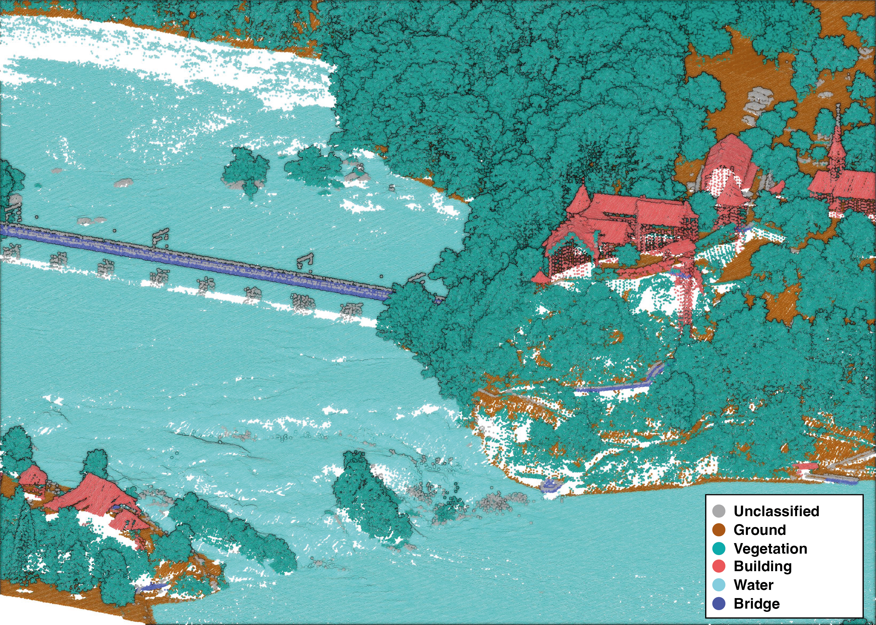
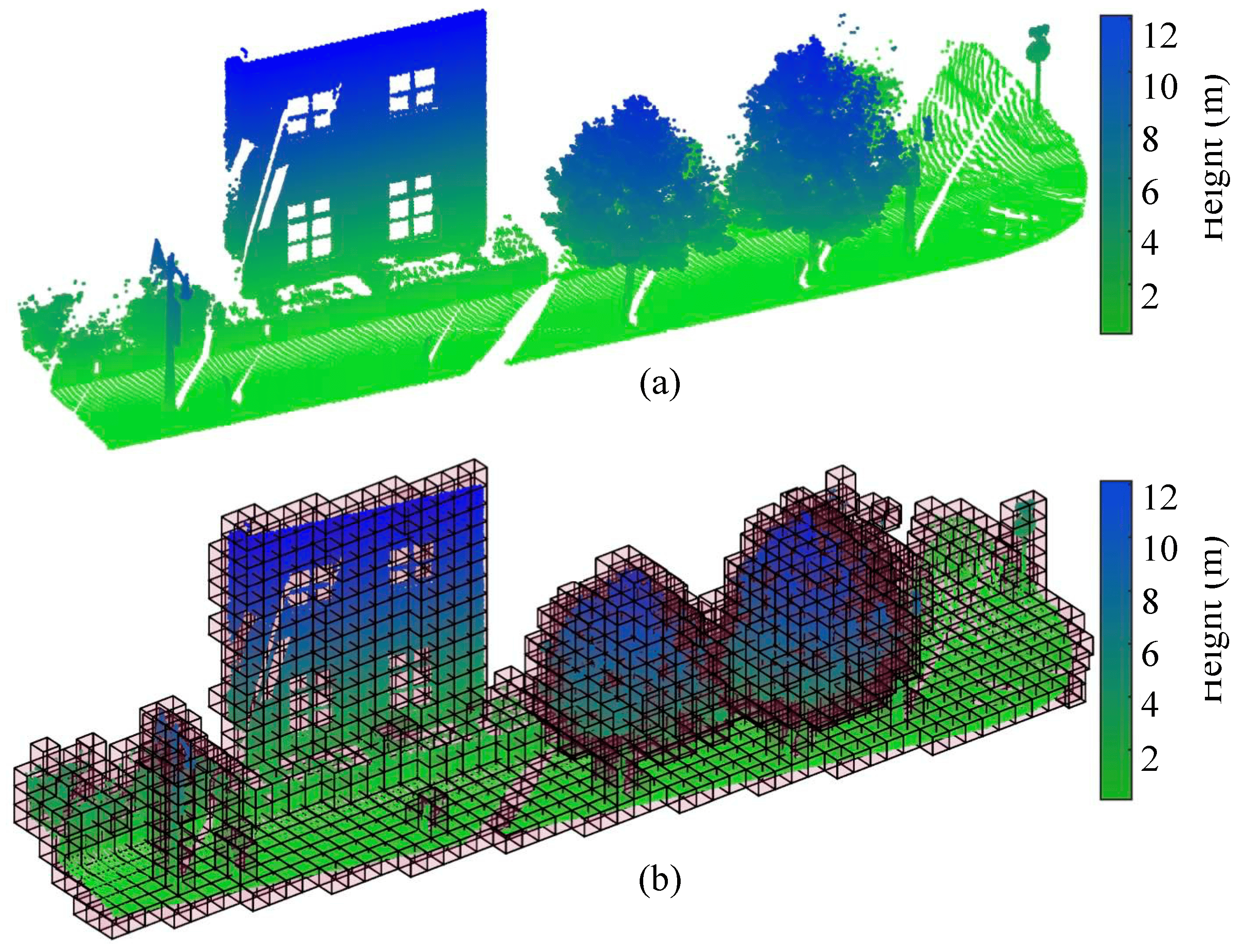
The usage of light detection and ranging (LiDAR) technology has seen a large increase in the field of geo-surveying over the recent years ¹. Data obtained from airborne acquisition provides rich 3D information about land cover in the form of a point cloud. These point clouds are typically processed after acquisition in order to assign a class to each point, as displayed in Figure 1.

Figure 1: View of the Rhine Falls in the classified point cloud of the product swissSURFACE3D.

To conduct their LiDAR surveys, the Federal Office of Topography (swisstopo) mandates external companies, in charge of the airborne acquisition and classification in post-processing. The process of verifying the quality of the data supplied is tedious, with an estimated duration of 42 working hours for the verification of an area of 216 km². A significant portion of this verification process is dedicated to ensuring the precision of the point classification. With the first generation of the LiDAR product ² nearing completion, swisstopo is keen to leverage the considerable time and effort invested to facilitate the quality assessment of the next generation. In this context, the swisstopo's LiDAR development team contacted the STDL to develop a change detection method.

As reviewed by Stilla & Xu (2023), change detection in point clouds has already been explored in numerous ways³. The majority of the research focus, however, on changes of geometry. Deep learning solutions are being extensively researched to apply the advancements in this field to change detection in point clouds⁴. However, to the best of our knowledge, no solution currently address the problem of change detection in the classification of two point clouds.
Most challenges of change detection in point clouds come from the unstructured nature of LiDAR data, making it impossible to reproduce the same result across acquisition. Therefore, the production of ground truth and application of deep learning to point clouds of different generations can be challenging. To overcome this, data discretization by voxelization has already been studied in several works on change detection in point clouds, with promising results⁵⁶.

The goal of this project is to create a mapping of the changes observed between two generations of point clouds for a common scene, with an emphasis on classification changes.
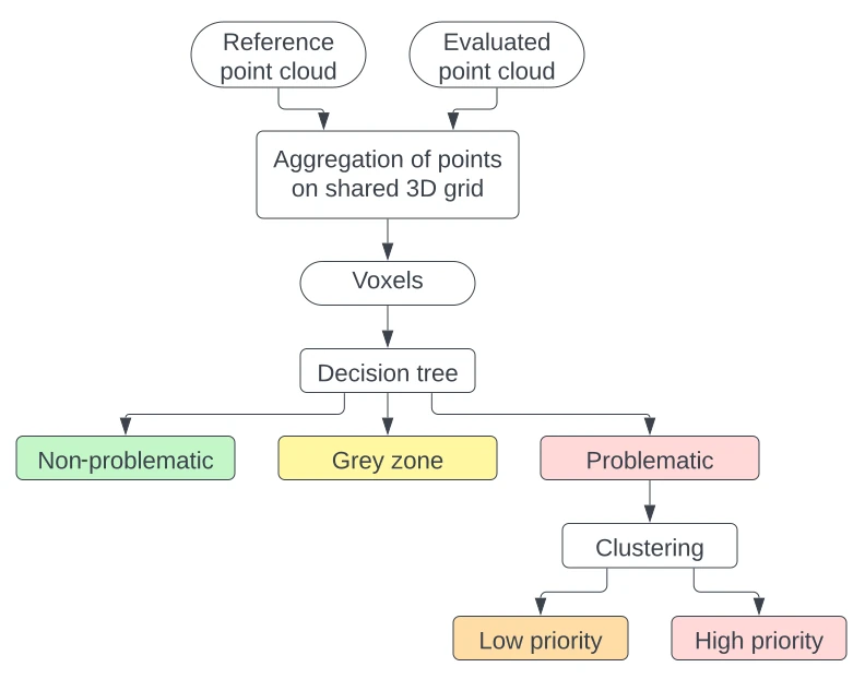
The proposed method creates a voxel map for the reference point cloud and the new point cloud for which classification was not controlled as thoroughly. By using the same voxel grid for both generations, direct comparisons can be performed on the occupancy of voxels by the previous and the new classes. Based on the domain expert's criteria, an urgency level is assigned to all voxels: non-problematic, grey zone or problematic. Problematic voxels are then clustered into high priority areas. The summarized process is displayed in Figure 2.

Figure 2: Overview of the workflow for change detection and assignment of a criticality level to the detected changes.

2. Data

2.1 LiDAR point clouds

The algorithm required two temporally distinct acquisitions for a same area. Throughout the document, we refer to the first point cloud as v.1. It served as reference data and is assumed to have a properly controlled classification. The subsequent point cloud, representing a new generation, is referred as v.2.

2.1.1 Choice of the LiDAR products

The swissSURFACE3D product was extensively controlled by swisstopo's LiDAR team before its publication. Therefore, its classification has the quality expected by the domain expert. It acted as the v.1, i.e as the generation of reference.

We thus needed to find some newer acquisition which fulfilled the following conditions:

• Availability in swissSURFACE3D: At the time of development, the initial classification control was not over for the whole of Switzerland. Point clouds were still in production at swisstopo for some cantons.
• Gap in acquisition dates: To have an exhaustive and representative panel of changes, point cloud of the v.2 had to be acquired at least two years apart from the v.1 data.
• Difference in density: The method aimed for robustness against changes in density, considering that advancements in technology lead to higher-quality sensors and an increased point density per square meter.
• Larger number of classes: Anticipating that swisstopo next iteration would introduce five additional classes, we required the v.2 point cloud to have a higher number of classes than in the v.1 point cloud. Furthermore, to be comparable, the v.2 classes needed to be subsets of the ones present in v.1.
• Typology of the point cloud: The selected point clouds needed to be acquired, at least partially, in an urban environment, where classification errors are more prevalent and, consequently, more control time is allocated.

For our v.2, we used the point cloud produced by the State of Neuchâtel, which covers the area within its cantonal borders. The characteristics of each point cloud are summarized in Table 1.

Table 1: Characteristics of swissSURFACE3D, used as v1, and the LiDAR product of the State of Neuchâtel, used as v2.

	swissSURFACE3D	Neuchâtel
Acquisition period	2018-19	2022
Planimetric precision	20 cm	10 cm
Altimetric precision	10 cm	5 cm
Spatial density	~15-20 pts/m2	~100 pts/m 2
Number of class	7	21
Dimension of one tile	1000 x 1000 m	500 x 500 m
Provided file format	LAZ	LAZ

2.1.2 Area of interest

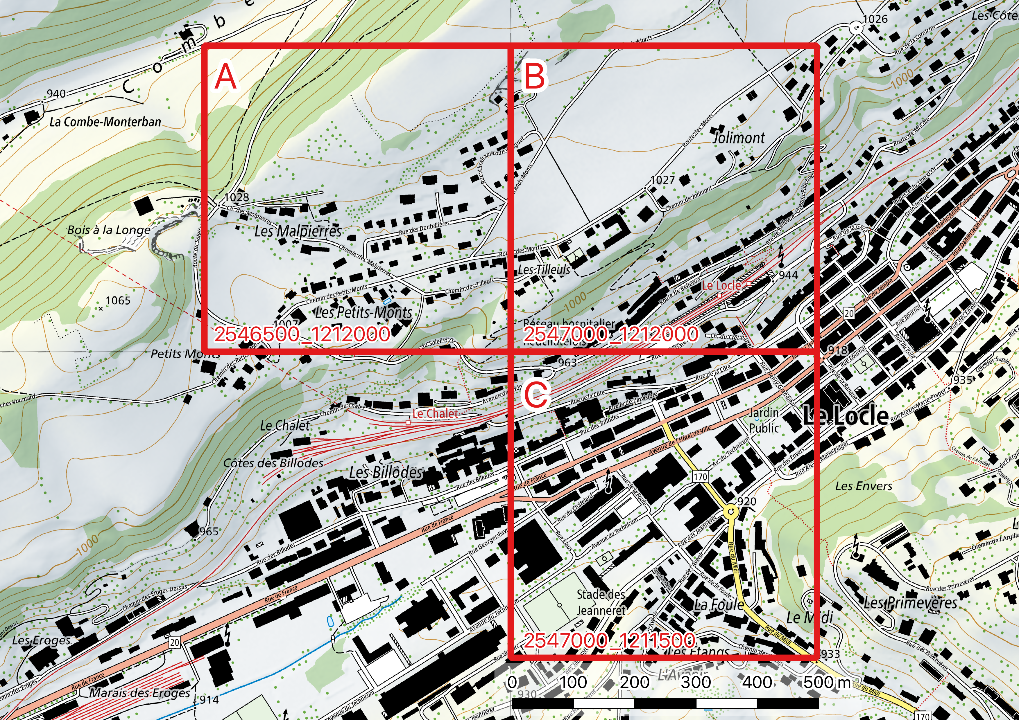
The delimitation of the LiDAR tiles used in this project is shown in Figure 3. We chose to work with tiles of the dimensions of the Neuchâtel data, i.e. 500 x 500 m. The tiles are designated by a letter that we refer to in the continuation of this document.

The tiles are located in the region of Le Locle. The zone covers an urban area, where quality control is the most time-consuming. It also possesses a variety of land covers, such as a large band of dense forest or agricultural fields.

Figure 3: Tiles used for the development of our method: A for a result control for the hyperparameter tuning, B for the choice of the voxel size and C for a control of the results by the domain expert.

2.2 Annotations by the domain expert

To understand the expected result, the domain expert controlled the v.2 point cloud in the region of Le Locle as if it was a new acquisition. A perimeter of around 1.2 km² was controlled.

The problematic zones were each defined by a polygon with a textual description, as well as the current and the correct class as numbers. A sample of annotations are shown in Figure 4.

Figure 4: Controlled area (left) and examples of control annotations within the detail zone, with the reported error as color and with the original and the corrected class as labels (right).

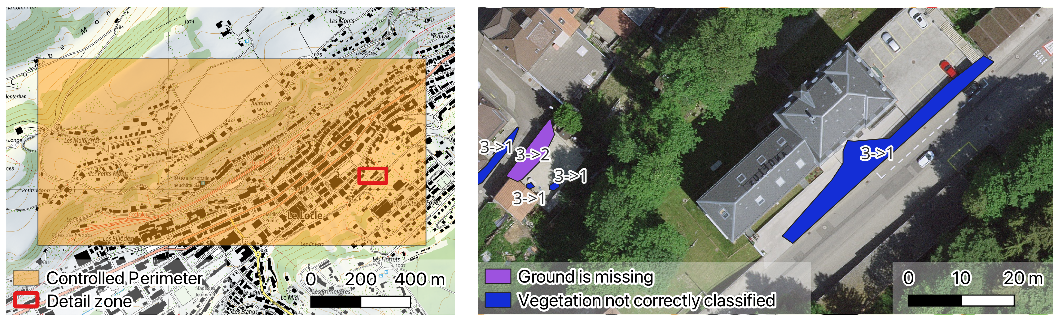
This provided us with annotations of areas where the point cloud data were incorrect. The annotations were used to calibrate the change detection.

It must be noted that this control was achieved without referring the v.1 point cloud. In this case we assume that the v.1 contains no classification error, and that the annotated areas therefore represent classification changes between the two generations.

3. Method

3.1 Correspondence between classes

To compare the classes between generations, we needed to establish their correspondence. We selected the classes from the swisstopo point cloud, i.e the reference generation, as the common ground. Any added classes in the new generation must come from a subdivision of an existing class, as explained in the requirements for the v.2 point cloud. This is the case with Neuchâtel data. Each class from Neuchâtel data was mapped to an overarching class from the reference generation, in accordance with the inputs from the domain expert. The details of this mapping are given in table 2. Notice that the class Ground level noise received the label -1. It means that this class was not treated in our algorithm and every such point is removed from the point cloud. This was agreed with the domain expert as this class is very different from the class Low Point (Noise) and doesn't provide any useful information.

Table 2: Mapping between the v.2 and v.1 point cloud. The field "original ID" provides the class number for v.2, the class name corresponds to the class description from the metadata, and the corresponding ID shows the class number from v.1 to which it is assigned.

Original ID	Class name	Corresponding ID
1	Unclassified	1
2	Ground	2
3	Low vegetation	3
4	Medium vegetation	3
5	High vegetation	3
6	Building roofs	6
7	Low Point (Noise)	7
9	Water	9
11	Piles, heaps (natural materials)	1
14	Cables	1
15	Masts, antennas	1
17	Bridges	17
18	Ground level noise	-1
19	Street lights	1
21	Cars	1
22	Building facades	6
25	Cranes, trains, temporary objects	1
26	Roof structures	6
29	Walls	1
31	Additional ground points	2
41	Water (synthetic points)	9

Figure 5: Reallocation of points from the v.2 classes (left) to the v.1 classes (right) for tile B with the class numbers from the second generation indicated between parenthesis.

As visible on Figure 5, seven classes were reassigned to class 1 Undefined. However, they represented a small part of the point cloud. The most important classes were ground, with in equal parts of ground and additional ground points, vegetation, with mainly points in high vegetation, and building, with mainly points on building roofs.

3.2 Voxelization of the point clouds

The method relies on the voxelization of both point clouds. As defined in Xu et al. (2021)⁷, voxels are a geometry in 3D space, defined on a regular 3D grid. They can be seen as the 3D equivalent to pixels in 2D. Figure 6⁸ shows how a voxel grid is defined over a point cloud.

Figure 6: Representation of a point cloud (a) and its voxel grid (b), courtesy of Shi et al. (2018).

3.2.1 Preprocessing of LiDAR tiles

It must be noted that the approach operated under the assumption that both point clouds were already projected in the same reference frame, and that the 3D positions of the points were accurate. We did not perform any point-set registration as part of the workflow, as the method focuses on finding errors of classification in the point cloud.

Before creating the voxels, the tiles were cropped to the size of the generation with the smallest tiling grid. Here, the v.1 tiles were cropped from 1000 x 1000 m to the dimensions of v.2, i.e 500 x 500 m. A v.2 tile corresponds exactly to one quarter of a v.1 tile, so no additional operations were needed.

3.2.3 Voxelization process

In the interest of keeping our solution free of charge for users, and to have greater flexibility in the voxelization process, we chose to develop our own solution, rather than use pre-existing tools.

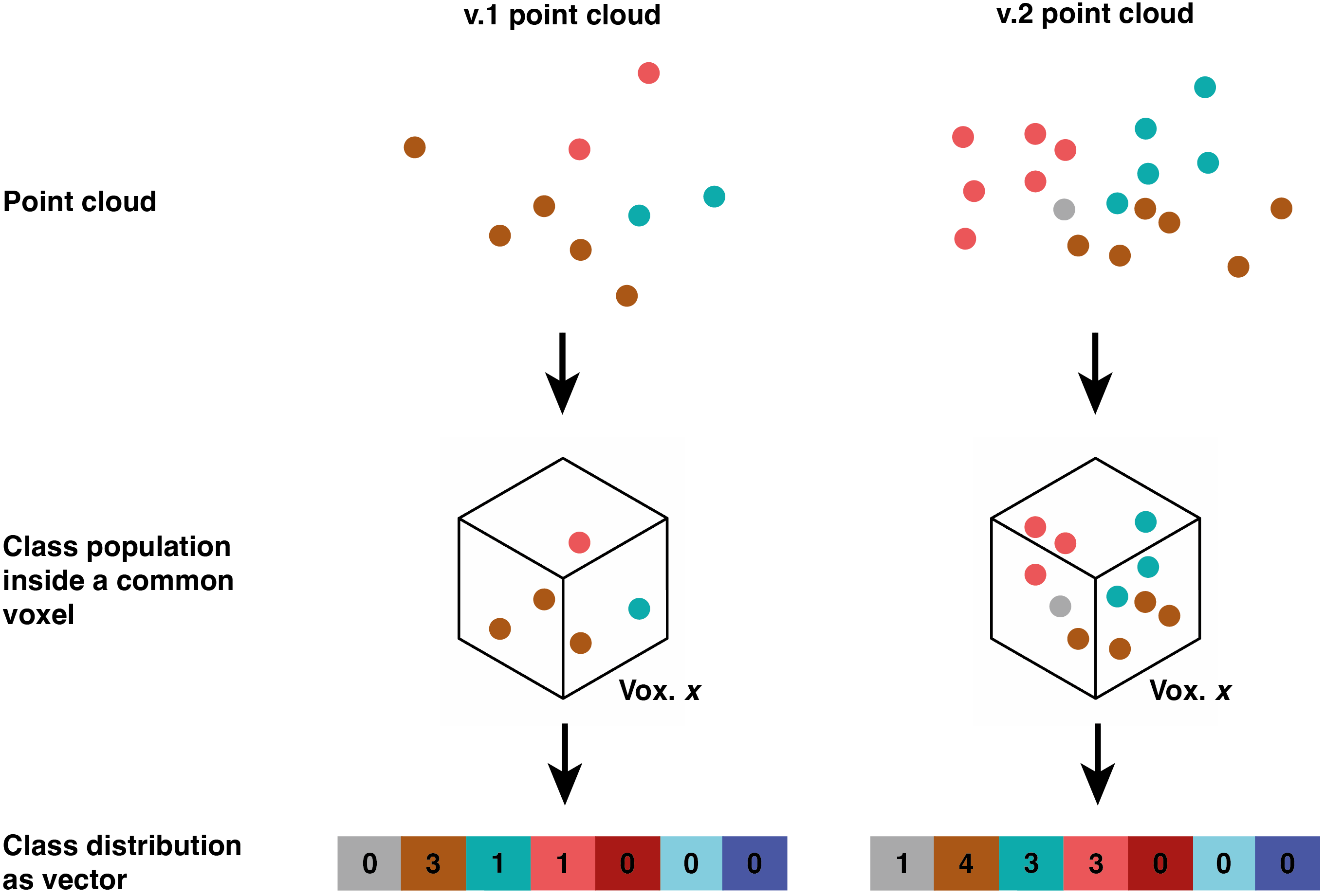
We used the python libraries laspy and pandas. Given a point cloud provided as a LAS or LAZ file, it returned a table with one row per voxel. The voxels were identified by their center coordinates. In addition, the columns provided the number of points for each class contained within the voxel for each generation. Figure 7 shows a visual representation of the voxelization process for one voxel element.

Figure 7: Summarized process for the creation of one voxel in the v.1 (left) and the v.2 (right) generation from the point cloud to the class distribution as a vector. The class distribution is saved for both generations in a table.

3.3 Determination of the voxel size

The voxels must be sized to efficiently locate area of changes without being sensitive to negligible local variations in the point location and density.

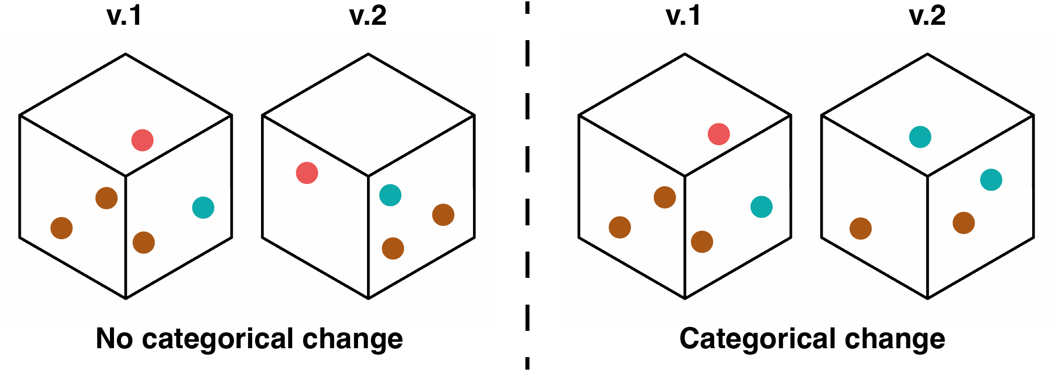
We assumed that although a point cloud changes between two generations, the vast majority of its features would remain consistent on a tile of 500 x 500 m. Following this hypothesis, we evaluated how the voxel size influenced the proportion of voxels not filled with the same classes in two separate generations. We called this situation a "categorical change". A visual example is given in Figure 8.

Figure 8: Example of a situation with no categorical change (left) and a second situation with a categorical change (right)

When the proportion of voxels presenting a categorical change was calculated for different voxel sizes, it rose drastically around a size of 1.5 m, as visible on Figure 9. We postulated that this is the minimum voxel size which allows observing changes without interference from the noisy nature of point clouds.

Figure 9: Proportion of categorical changes for different voxel size in tile B. The horizontal axis is the voxel size. The vertical axis represents the percentage of voxels experiencing a categorical change between the two generations. 

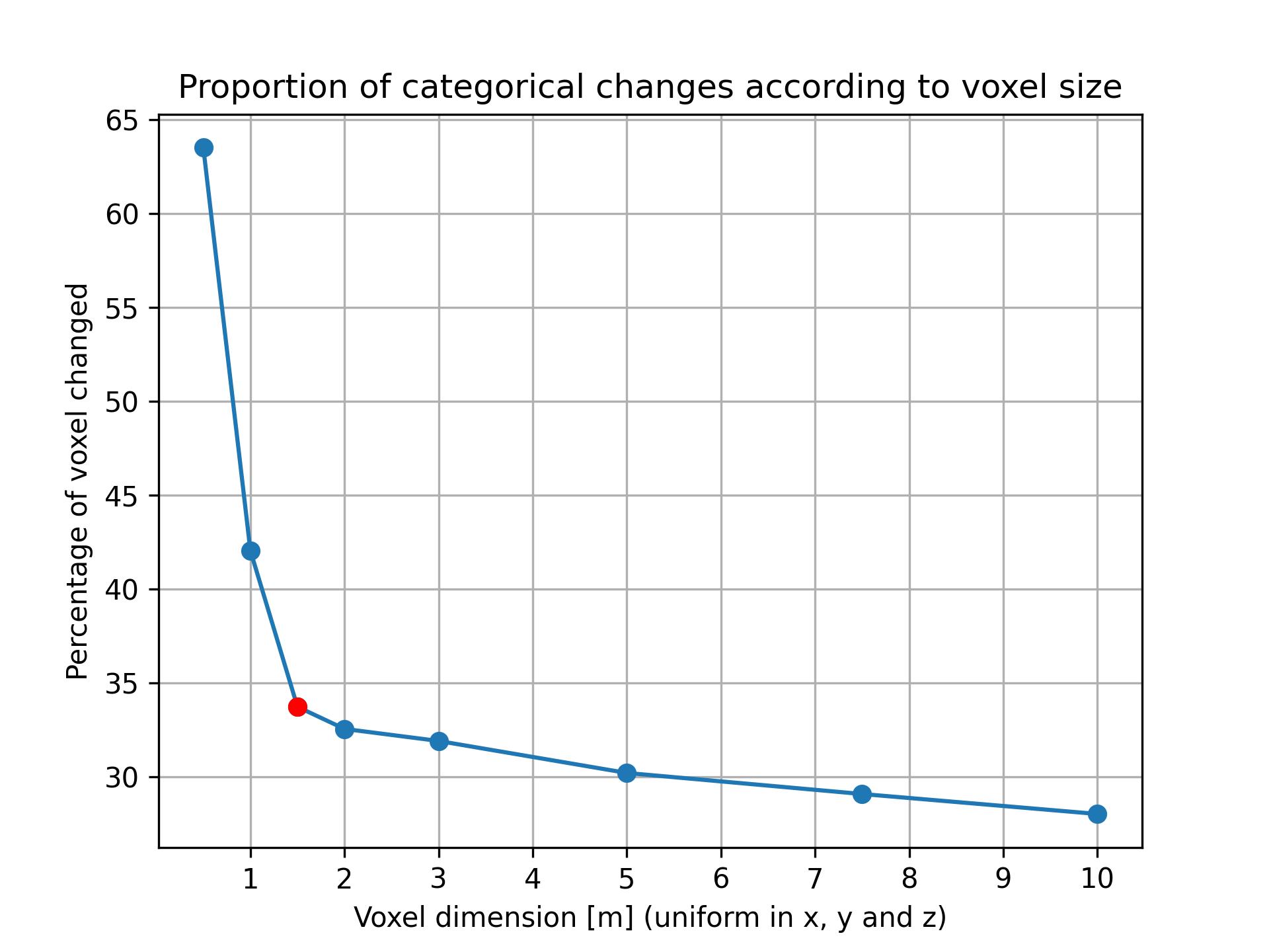
For the rest of the development process, square voxels of 1.5 m are used. However, the voxel width and height can be modified in the scripts if desired.

3.4 Criticality tree

The algorithm must not only detect changes, but also assign them a criticality level. We translated the domain expert's criteria into a decision tree, which sorts the voxels into different criticality levels for control. The decision tree went through several iterations, in a dialogue with the domain expert. Figure 10 provides the final architecture of the tree.

Figure 10: Decision tree used to classify the voxels based on the different types of changes and their criticality.

The decision tree classifies the voxels into three buckets of criticality level: "non-problematic", "grey zone" and "problematic".

• "non-problematic" voxels have little to no change. No control is necessary.
• "Grey zone" voxels undergo a change that is coherent with their neighbors or due to the presence of the class 1, i.e. the Undefined class, in the new generation. The detected changes should not be problematic, but might be interesting to verify in the case of a very thorough control.
• "Problematic" voxels are the ones with important changes such as strong variations in the class proportions or changes not reflected in their neighborhood. They are relevant to control.

Let us note that although only three final buckets were output, we preserved an individual number for each outgoing branch of the criticality tree, as they provided a more detailed information. Those numbers are referred as "criticality numbers".

The decisions of the criticality tree are divided into two major categories. Some are based on qualitative criteria which is by definition true or false. Others, however, depend on some threshold which had to be defined.

3.4.1 Qualitative decisions

Decision A: Is there only one class in both generations and is it the same?
Every voxel that contains a single, common class in both generations is automatically identified as non-problematic.

Decision B: Is noise absent from the new generation?
Any noise presence is possibly an object wrongly classified and necessitates a control. Any voxel containing noise in the new generation is directed to the "problematic" bucket.

Decision G: Is the change a case of complete appearance or disappearance of a voxel?
If the voxel is only present in one generation, it means that the voxel is part of a new or disappearing geometry that might or not be problematic, depending on decisions H and J.
If the voxel is present in both generations, we are facing a change in the class distribution due to new classes in it. The decision I will compare the voxel with its neighbors to determine if it is problematic.

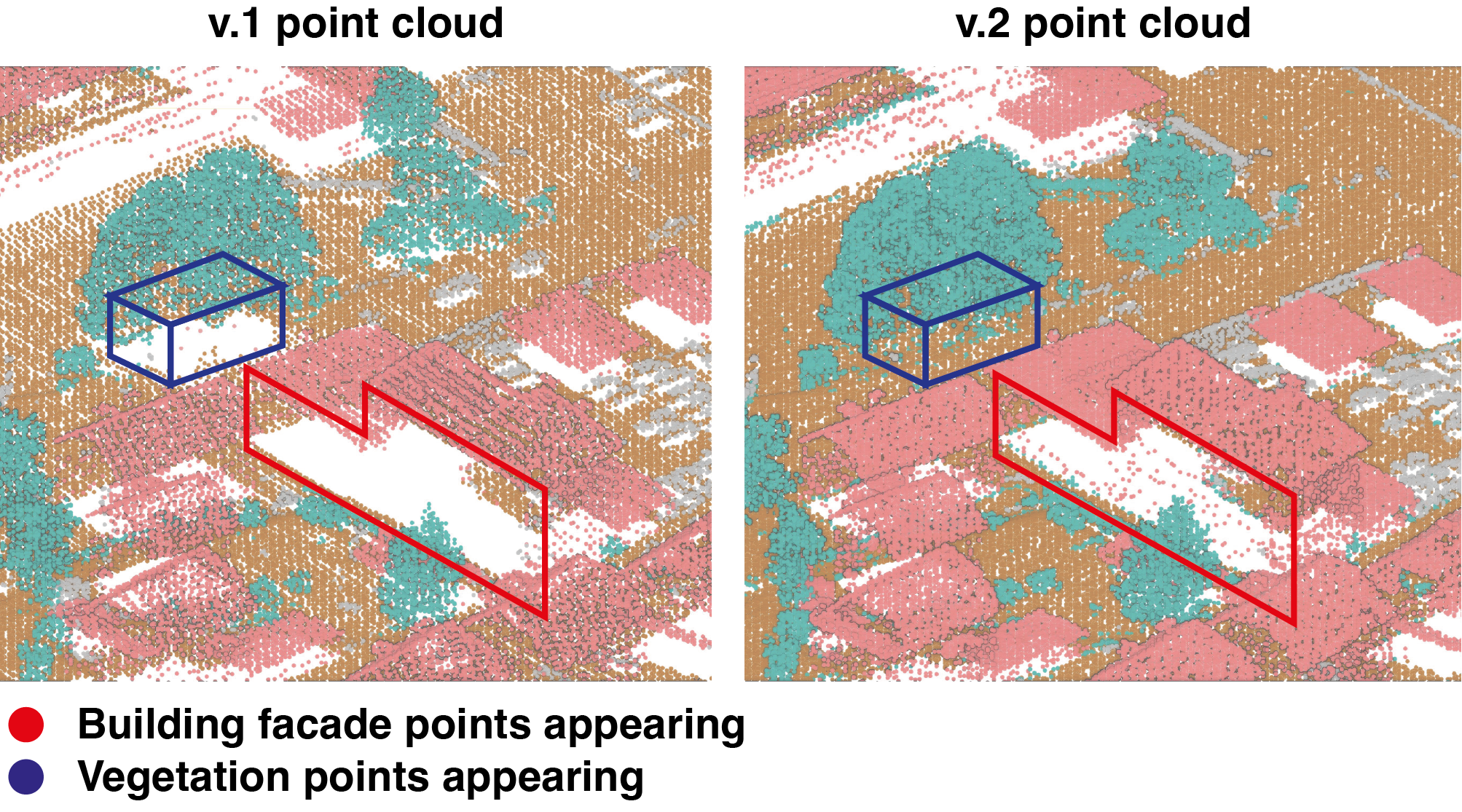
Decision J: Is it the specific case of building facade or vegetation?
Due to the higher point density in the v.2 point cloud, point proportions may change in voxels compared to the v.1 point cloud, even though the geometry already existed. We particularly noticed this on building facades and under dense trees, as shown in the example given in Figure 11. To avoid classifying these detections as problematic, a voxel with an appearance of points in the class building or vegetation is not problematic if it is located under a non-problematic voxel containing points of the same class.

Figure 11: Example of non-problematic appearance of points in the v.2 point cloud due to the difference of density between the two generations.

3.4.2 Threshold based decisions

The various thresholds were set iteratively by visualization of the results on tile A and visual comparison with the expert's annotations described in section 2.2. Once the global result seemed satisfying, we assessed the criticality label for a subset of voxels. Eight voxels were selected randomly for each criticality number. Given that there are 13 possible outcomes, 104 voxels were evaluated. A first evaluation was performed on tile A without the input of the domain expert. It allowed for the hyperparameter tuning. A second evaluation was conducted by the domain expert on tile C and he declared that no further adjustment of the threshold was necessary.

Cosine similarity

The decision C, D and E require to evaluate the similarity between the distribution of the previous and the new classes occupying a voxel. We thus sought a metric adapted to compare the two distributions. Many ways exist to measure the similarity between two distributions⁹. We settled for the well-known cosine similarity. Given two vectors X and Y, it is defined as: \(\text{Cosine Similarity}(\mathbf{X}, \mathbf{Y}) = \frac{\mathbf{X} \cdot \mathbf{Y}}{\|\mathbf{X}\| \|\mathbf{Y}\|}\)

This metric measures the angle between two vectors. The magnitude of the vectors holds no influence on the results. Therefore, this measure is unaffected by the density of the point clouds. The more the two vectors point in the same direction, the closer the metric is to one. Vectors having null cosine similarity correspond to voxels where none of the classes present in the previous generation match those from the new one.

One limitation of the cosine similarity is its requirement for both vectors to be non-zero. For cases where a voxel is only occupied in a single generation, an arbitrary cosine similarity of -1 is set.

Decision C: Does the proportion of class stay similar and the classes don't change?
We assessed whether the proportion of class stays similar between generations. A threshold of 0.8 is set on the cosine similarity.

flowchart LR
    A[Prev. gen.<br> 0 &#124 0 &#124 4 &#124 2 &#124 0 &#124 0 &#124 7] --> E(Cosine similarity)
    B[New gen.<br> 25 &#124 0 &#124 20 &#124 0 &#124 0 &#124 5 &#124 40] --> E

    E-->F[0.84]

Graph 1: Example of vectors and their resulting cosine similarity when considering all the classes.

Decision D: Do the previous classes keep the same proportions?
We computed the cosine similarity based only on the vector elements which are non-empty in the previous generation. A threshold of 0.8 is set as the limit.

Let us note that voxels present only in one of the two generations are here artificially considered to retain the same class proportion. They are treated further down the decision tree by the decision G.

flowchart LR
    A[Prev. gen.<br> 0 &#124 0 &#124 4 &#124 2 &#124 0 &#124 0 &#124 7] --> C[4 &#124 2 &#124 7]
    B[New gen.<br> 25 &#124 0 &#124 20 &#124 0 &#124 0 &#124 5 &#124 40] --> D[20 &#124 0 &#124 40]
    C-->E(Cosine similarity)
    D-->E
    E-->F[0.97]

Graph 2: Example of vectors and their resulting cosine similarity when considering only the classes present in the reference generation v.1.

Decision E: Is the change due to the class 1?
We assessed whether the change is due to the influence of the unclassified points (class 1). To do so we computed the cosine similarity with all vector elements except the first one, corresponding to unclassified points. If the cosine similarity was low when considering all vector elements (decision C), but high when discarding the quantity of unclassified points, this indicates that the change is due to class 1. A threshold of 0.8 is set as the limit.

flowchart LR
    A[Prev. gen.<br> 0 &#124 0 &#124 4 &#124 2 &#124 0 &#124 0 &#124 7] --> C[0 &#124 4 &#124 2 &#124 0 &#124 0 &#124 7]
    B[New gen.<br> 25 &#124 0 &#124 20 &#124 0 &#124 0 &#124 5 &#124 40] --> D[0 &#124 20 &#124 0 &#124 0 &#124 5 &#124 40]
    C-->E(Cosine similarity)
    D-->E
    E-->F[0.96]

Graph 3: Example of vectors and their resulting cosine similarity when excluding the first class.

Decision F: Is class 1 presence low in the new generation?
In the case where the change is due to the unclassified points, we wished to evaluate whether such points are in large quantity in the new voxel occupancy. Because the number of points is dependent on the density of the new point cloud, we cannot simply set a threshold on the number of points. To solve this issue, we normalize the number of unclassified points in the voxel, \(n_{unclassified}\). Let \(N_{reference}\) and \(N_{new}\) be the total number of points in the v.1 and v.2 point cloud respectively. The normalized number of unclassified points \(\tilde{n}_{unclassified}\) is defined as:

\[\tilde{n}_{unclassified}= n_{unclassified}\cdot \frac{N_{reference}}{N_{new}} \]

An arbitrary threshold of 1 is set as the limit on \(\tilde{n}_{unclassified}\). Under this threshold, the presence of the class 1 was considered as low in the new generation.

Decision H & I: Do the neighbor voxels share the same characteristics?
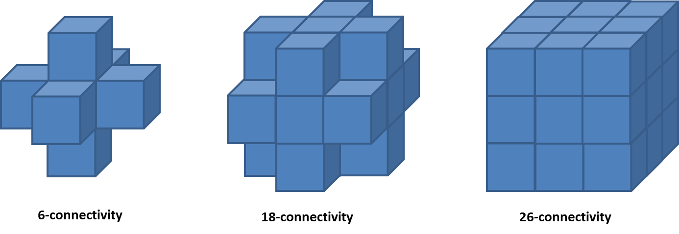
For both decisions we searched the neighbors of a given voxel to evaluate if they share the same characteristics. To make the search of these neighbors efficient, we built a KD-Tree from the location of the voxels. For each voxel, it then assessed whether the neighbors shared the same classes or not. Each class of the evaluated voxel must be present in at least one neighbor. The radius of search influences the number of voxels used for comparison. Let \(x\) be the voxel edge length, using search radii of \(x\), \(\sqrt{2}x\) or \(\sqrt{3}x\) leads to considering 6, 18 or 26 neighbors respectively, as displayed in Figure 12¹⁰. Note that the radius is not limited to these options and search among further adjacent voxels is possible.

Figure 12: Possible connectivity types to define the neighborhood of a voxel from the website brainvisa.info.

In the case where the voxel is only present in one generation, i.e for the decision H, the neighbors considered are the following:

• appearance of the voxel: the class distribution of the new voxel is compared to the voxels of the reference generation. Therefore, the extension of a neighboring class to the new voxel is non-problematic, whereas the appearance of a whole new geometry is classified in the grey zone.
• disappearance of the voxel: the class distribution of the old voxel is compared to the voxels of the new generation. Therefore, shrinking a geometry to cover only the neighboring voxels would be non-problematic, whereas the disappearance of a entire geometry is classified in the grey zone.

In the case where the class distribution changes due to new classes present in the voxel compared to v.1, i.e for the decision I, the class distribution of the voxel in v.2 will be compared to its neighbors in v.2. Therefore, if the entire area share the same classes, the voxel is classified the grey zone, but if the change is isolated, it goes into the "problematic" bucket.

3.4.3 Description of the "grey zone" and "problematic" buckets

We provide a brief description of the output for each branch of the decision tree ending in the grey zone and problematic buckets. They are identified by their criticality number. Let us note that the criticality numbers are not a ranking of the voxel priority level for a control, but identifiers for the different types of change.

• Grey zone:

  • 7: Appearance of a voxel or change in the class proportions due to unclassified points in the new generation;
  • 8: Change in the class distribution due to extra classes present in the voxel. The neighboring voxels share the same class occupancy.

• Problematic:

  • 9: Disappearance, i.e. a voxel which contains points in v.1 but not in v.2. The neighboring voxels do not show the same change;
  • 10: Appearance, i.e. a voxel which contains no points in v.1 but is filled in v.2. The neighboring voxels do not show the same change;
  • 11: Change in the class distribution due to extra classes present in the voxel. The neighboring voxels do not share the same class occupancy;
  • 12: Changes in the distribution for old and new classes present in the voxel between the v.1 and v.2 occupancy;
  • 13: Presence of points classified as noise in v.2.

3.5 Clustering of problematic voxels

Voxels ending in the "grey zone" and "problematic" buckets were often isolated. This creates a noisy map, making its usage for quality control challenging. To provide a less granular change map, we chose to cluster the change detections, highlighting only areas with numerous problematic detections in close proximity. In practice, we leveraged the DBSCAN algorithm. Then, the smallest clusters were filtered out and their cluster number is set to one. They are not treated as clusters in the rest of the processing. The hyperparameters for the clustering process are shown in Table 3. They were determined by the expert through the visualization of the results. The epsilon parameter was chosen to correspond to a neighborhood of 18 voxels, as illustrated on Figure 12.

Table 3: Hyperparameters used for the DBSCAN clustering and the filtering of the clusters.

Hyperparameter	Description	Value
Epsilon	radius of the neighborhood for a given voxel in meters	2.13
Minimum number of samples	minimum number of problematic voxels in the epsilon neighborhood for a voxel to be a core point for the cluster	5
Minimum cluster size	minimum number of voxels needed inside a cluster for it to be preserved	10

The clusters should be controlled in priority; they form the primary control. Voxels outside a cluster go into the secondary control as illustrated in the schema of the workflow on Figure 13. Their cluster number of those voxels is set to zero.

Figure 13: Schema of the additional step of clustering for the problematic voxels and assignment of the voxels falling inside a cluster to the primary control.

All problematic voxels went through this DBSCAN algorithm at once, without distinction based on the criticality number. That way, detections related to the same geometry were grouped together even if its voxels are not all labeled with the same criticality number. In the end, the label which was the most present inside a cluster is attributed to it.

3.6 Visualization of detections

Several possibilities were considered for the visualization of the results, as shown in Figure 14.

Figure 14: Comparison of a voxel mesh in green (a), a LAS point cloud (b), and a shapefile with the most represented criticality number of the cluster (c) for the visualization of the detections. The cluster in the point cloud and shapefile are colored in orange and blue depending on their criticality number. The v.2 point cloud is visible as background.

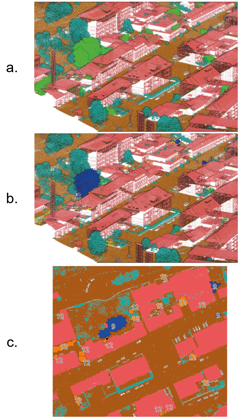
Table 4 shows the advantages and drawbacks of the different methods. In the end, the domain expert required that we provide the results as a shapefile.

Table 4: Comparison of the visualization methods

	Voxel mesh	LAS point cloud	shapefile
2D representation of the space occupied by voxels	Yes	No	Yes
3D representation of the space occupied by voxels	Yes	No	No
Visualization of the voxel height	Yes	Yes	No
Numerical attributes	No	Yes	Yes
Textual attributes	No	No	Yes

4. Results

4.1 Granularity of results

Figure 15 shows the voxels produced by the algorithm for the different priority levels. From the base with all the created voxels, each level reduces the number of considered voxels. At the last level, the clustering effectively reduces the dispersion of voxels, keeping only clearly defined groups.

Figure 15: Voxels by their center coordinates in a point cloud for the different levels of priority for tile C. Going from the clustered detections at the top to all the voxels at the bottom.

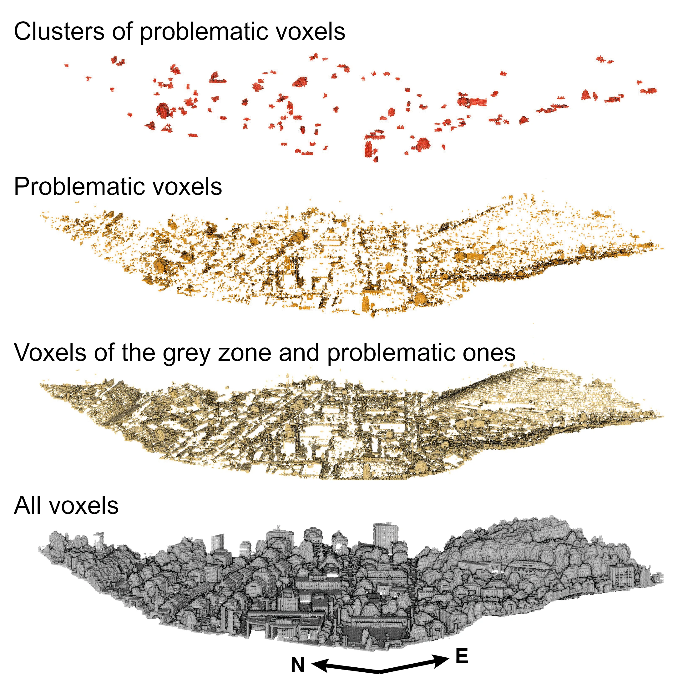
Table 5 gives the number and percentage of voxels retained at each level. For tile C, the voxels falling into the "grey zone" and the "problematic" buckets represent 14.86% of all voxels. If only the problematic ones are retained, this percentage is reduced to 4.77%. Finally, after removing the voxels which do not belong to a cluster, only 2.30% remains.

Meanwhile, the covered part of the tile decreases from 35.80% with all the problematic voxels and the ones of the grey zone, to 11.89% with only the problematic voxels, and to 4.53% with only the clustered voxels. In the end, an expert controlling the classification would have to check in priority 5% of the total tile area.

Table 5: Number of voxels preserved in each urgency level on tile C.

Urgency level	Number of voxels	Percentage of all voxels	Covered tile area
Clustered detections	8'756	2.30 %	4.53 %
Problematic detections	18'146	4.77 %	11.89 %
Problematic + grey zone detections	56'363	14.83 %	35.80 %
All voxels	380'165	100 %	100 %

The percentage of voxels and covered tile area decrease consequently between each granularity level. The higher the granularity is, the larger the difference in the voxel number and the covered area between two levels. The covered tile area decreases more slowly than the percentage of voxels retained.

4.2 Distribution of the decision tree outcomes

4.2.1 Distribution of the points in the criticality numbers and buckets

Figure 16 shows the percentage of points from the new point cloud coming out of each branch of the decision tree. The distribution between criticality buckets is given at the top of the figure. The vast majority of points belongs to non-problematic voxels, with around 80% of them being from the first tree branch. This corresponds to the case where only one class is present in both generations. We notice that 10% of the points end up in voxels assigned to the grey zone. It is mostly due to the output of the 8^th tree branch. For this specific tile, 1.81% of points from the new point cloud end up in problematic voxels. Let us note that no point ends up in voxels with the 4^th and 9^th criticality number. This is because those correspond to case of geometry disappearances.

Figure 16: Relative distribution of the points from the new point cloud depending on the criticality number and bucket of their voxel. Results for tile A.

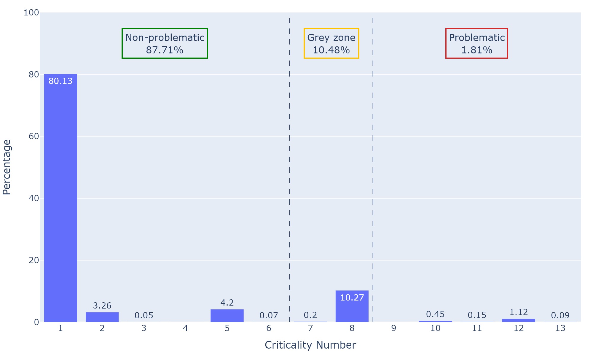
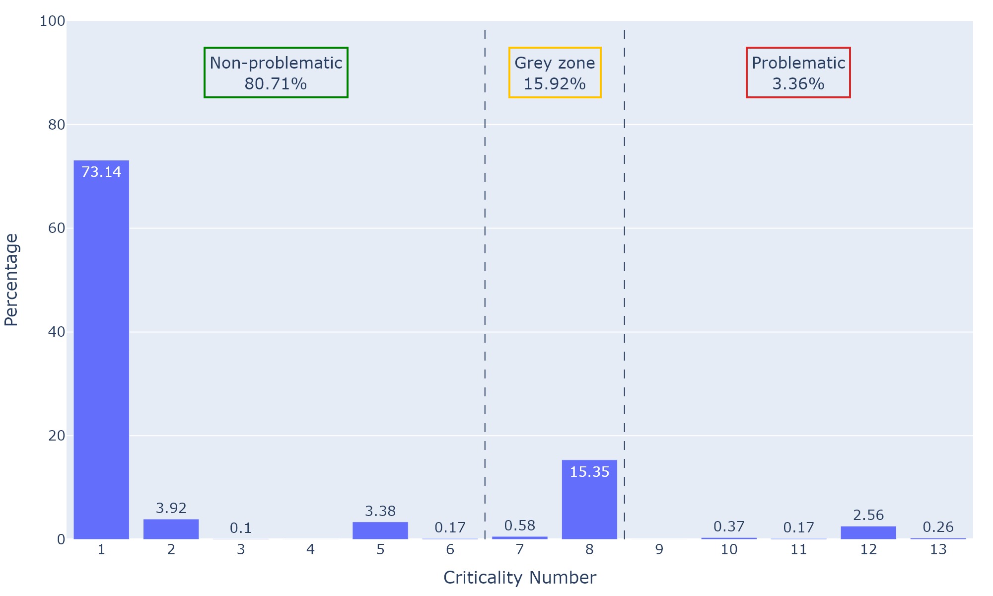
Figure 17 shows the same plot, but with the v.1 point cloud for tile C. In that case the percentage of non-problematic points is smaller than for tile A, with more points falling in the "grey zone" and "problematic" buckets, but the overall trend stays similar. The only changes over 1% are for criticality numbers 1 (-6.99 points), 8 (+5.08 points), and 12 (+1.44 points). Fewer voxels present one same class across generations, marked with the criticality number 1. More voxels present a change in the distribution. This change can be non-problematic if due to the presence of extra classes in the voxel and reflected by the neighboring voxels (criticality number 8). It is problematic if there is a drastic change in the distribution of all classes in the voxel (criticality number 12).

Figure 17: Relative distribution of the points from the new point cloud depending on the criticality number and bucket of their voxel. Results for tile C.

4.2.2 Distribution of the criticality numbers in the clusters

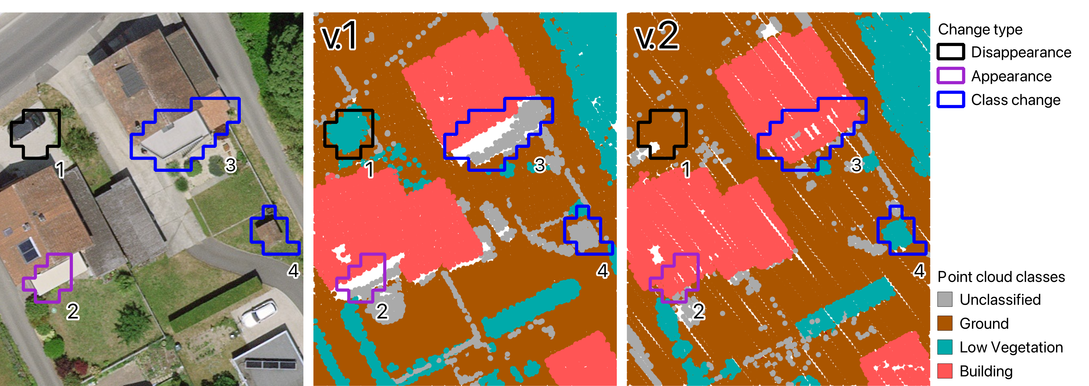
Figure 18 displays a sample of clusters as an example. These are shown as a shapefile, which is the visualization format required by the domain expert. One cluster (#1) indicates the disappearance of a tree. Another cluster (#2) designates an appearance. Upon closer examination, the voxels contributing to the cluster comprise different types: "appearance" and "class change". The most present label is assigned to the cluster. Finally, two zones with differences in classification are highlighted: one (#3) for a building structure going from class unclassified to building, and the other (#4) for a shed going from unclassified to vegetation.

Figure 18: Example of resulting clusters with the corresponding point cloud for the reference generation (v.1) and the uncontrolled generations (v.2).

The 8'756 problematic voxels for the primary control are grouped in 263 individual clusters. The repartition of clusters and voxels among the criticality numbers is given in Table 6. Among the clusters, 67% of them contain mostly voxels with the criticality number 12, meaning that there is a major change in the class distribution for the delineated area. Then, 13% and 12% of the voxels are dominated by a geometry appearance and disappearance respectively. Only 7% of the clusters contain in majority an occurrence of the noise class. It is normal that no cluster is tagged with the criticality number 11, because it is assigned by definition to isolated class changes.

The criticality number 12 is the most present criticality number among the clustered voxels. However, its percentage decrease of 18 points at the voxel scale compared to the cluster scale. On the other hand, the presence of the criticality number 8 increase by 15 points at the voxel scale compared to the cluster scale. The other percentages remain stable.

Table 6: Number of clusters and number of voxels in the primary control for each criticality number on tile C.

Criticality number and its description	Distribution in the clusters	Distribution in the voxels in the primary control
9. Appearance of a geometry	13.31 %	27.91 %
10. Disappearance of a geometry	12.17 %	16.47 %
11. Isolated minor class change	0 %	0.13 %
12. Major change in the class distribution	67.30 %	49.63 %
13. Noise	7.22 %	5.86 %

4.2.3 Distribution of the LiDAR classes in the criticality buckets

Figure 19 shows the distribution of the LiDAR classes in the criticality buckets. We see that for the three main classes of this tile, ground, vegetation and building, the vast majority of points fall in non-problematic voxels, with the ground class having a higher proportion of points falling in "grey zone" voxels than the others. Unclassified points fall predominantly in the grey zone voxels. The grey zone gets a lot of voxels due to the decision C of the criticality tree, which requires that the voxels share the same classes in both generations. It is difficult for voxels to end up in the "non-problematic" bucket, if they did not pass the decision C.
All points classified as noise end up in the problematic bucket, as required by the domain expert.
Finally, points from the bridge class fall in "problematic" and "grey zone" voxels. This class is, however, in very low quantity in the new point cloud (only 0.014% of all points) and is thus not statistically significant.

Figure 19: Distribution of the points among criticality bucket relative to their LiDAR class, as well as the percentage represented by the class in the point cloud. Let us note the results are for the v.2 point cloud on tile C and that no point was classified as water for this tile.

4.3 Assessment of a subset of detections

As mentioned in section 3.4.2, 104 voxels were evaluated on tile C, i.e 13 per criticality number. Per the expert review, all the non-problematic and "grey zone" voxels were deemed rightfully attributed. However out of the 40 selected problematic voxels, nine detections did not justify their status. Three of those were for cases of appearance and disappearance of geometry. Out of those, two were due to an isolated change of density in the area of the voxel, a situation which can occur in vegetated areas. The other six came from the tree branch 11, which detects small changes that are not present in the neighboring voxels. After discussion with the domain expert, it was agreed that such changes still needed to be classified as problematic, but due to their isolated nature, would not be checked as a priority. After the implementation of the clustering via the DBSCAN algorithm, these voxels of criticality number 11 and isolated changes in vegetation are filtered out.

5. Discussion

5.1 Interpretation of the results

In Section 4.1, the voxel count for the different granularity levels highlights the number of detections that would have to be controlled at each level. For the clustered detections, which would be the principal mapping to use, only 2.30% of all evaluated voxels are to be controlled. It represents 4.53% of the tile area. The domain expert confirmed that the final amount of voxel to control is reasonable and would allow saving resources compared to the actual situation.

For each granularity level, the percentage of the tile area covered is 2 to 3 times higher than the percentage of voxels considered. It means that between each granularity level, a part of the eliminated voxel does not impact the covered tile area. The reason must be that the area is a 2D measurement while the voxels are positioned in the 3D space and can cover the same area by belonging to the same grid column. The voxels of a same column must be frequently assigned to different criticality buckets. Therefore, the covered tiles area decreases more slowly than the percentage of voxels considered.

From the results obtained in Section 4.2.1, we see that the vast majority of points from the new point cloud end up in non-problematic voxels. The number of points falling in problematic voxels is limited, which is desired as a high quantity of problematic detections would not help in making the quality assessment faster. We notice, however, a relatively large number of points falling in voxels classified as "grey zone", due to the 8^th tree branch. These voxels typically exhibit high similarity in their distribution between the v.1 and the v.2, but do not retain precisely the same classes. The decision C will therefore exclude them from a quick assignment to the non-problematic voxels. Such a situation occurs, for example, if a few points of vegetation appear in a zone previously filled only with ground points. This situation generally isn't a classification error and reflects the reality of the terrain. However if it were to be a widespread problem of classification, it needs to be raised to the controller. This is why we preserve those rules which lead to a lot of "grey zone" detections instead of redirecting them to "non-problematic".

In Section 4.2.1, results are presented for tile A and C on Figures 16 and 17 respectively. Tile A has fewer voxels in the "problematic" and "grey zone" buckets than tile C. It is in accordance with our expectation than urban zones would have more detected changes, as they evolve faster than other areas and have some complex landscape to classify.

The numbers of Section 4.2.2 show that the majority of clusters and the majority of the voxels in clusters have the criticality number 12, indicating a major change in the class distribution. It is a satisfying point as the variations of the classification across generations were the main focus of this work. Let us not, however, that they dominate 67% of the clusters, but only 50% of the voxels in clusters are assigned to this criticality number. On the other hand, the criticality number 9, standing for the appearance of a geometry, represents 28% of the voxels present in clusters while it was only 13% of the clusters. Two possibilities can explain that: the clusters with a geometry appearance are larger than the ones with a major change in the class distribution, or this type of voxel is more present in clusters that were assigned to another criticality number.

Results of Section 4.2.3 show that the points of the three main LiDAR classes are assigned predominantly to the "non-problematic" bucket, which makes the map usable.
For the unclassified points, the majority are deemed in "grey zone". Because these points regroup, among other things, mobile and temporary objects, it is not desirable that every such appearance or disappearance ends up in the primary control. However, geometries which transform from a given class to unclassified, or the opposite, are problematic. That situation happens quite often, as indicated by the 17.43% of points ending in this level.
For the bridge class, none of the points fall in "non-problematic" because, in this specific tile, a small zone was classified as bridge in v.2 but no point of that class is present in v.1.

Finally, from the evaluation by the domain expert described in Section 4.3, we understand that the voxels are correctly classified into their criticality level, except for some minor cases. Some of the problematic voxels were not rightfully attributed. Even so, six out of nine of those voxels had the criticality number 11, whose detections are removed when applying the clustering. This sample evaluation instills confidence that the level of urgency attributed to the voxels corresponds well to the situation contained within, making it relevant for usage in a control of the classification.

5.2 Discussion of the results

As seen in the previous section, the proposed method generates a somewhat reasonable amount of problematic detections, accompanied by a considerable volume of instances falling within the "grey zone". The map for this intermediate level may not be suitable for initial quality control but can offer a more detailed delineation for precise assessment. The map of non-problematic voxels could also be used to highlight the areas requiring no quality assessment given the absence of changes in the distribution.

The proportion of points identified as problematic is very low (1-4%). However, their visual representation can be overwhelming for the controller, given the high number of scattered detections. To address this challenge, we introduced the clustering and filtering of detections. Though this allows for visually more understandable areas, it naturally sacrifices the exhaustiveness of the detections. For example, low walls and hedges were frequently classified differently between the v.1 and the v.2. Due to the clustering favoring areas with grouped elements, such elongated and thin objects can be cut out of the mapping. Possible future works could study other filtering methods to attenuate this issue.

Currently, no full assessment of the detections on a tile was performed. Therefore, it is hard to estimate the quantity of detections that would be missing in clusters or in the "problematic" bucket.

For the precision of the results, the evaluation of the small subset of detections by the domain experts indicates that they are relevant and possibly useful as a tool for quality assessment.

While the developed method allows for finding changes between two point clouds, it has some limitations. First, it only works if the classes from v.2 can be mapped to overarching classes in v.1. This is not always the case, due to the lack of consensus between LiDAR providers. Another limitation comes from the voxel size. Indeed, by employing fixed volumes of 3.375 m³ to detect the changes, points not contributing to the actual change will also be included in the highlighted areas. A possible improvement would be to refine the detection area after the clustering. Another thing to consider is that the method work on a single tile at a time, without consideration of the tiles around it. This can potentially affect the clustering step as voxels on the border have fewer neighbors. To ensure that this does not affect the results a buffer could be taken around the tile. This buffer could also ensure that the total tile size is a multiple of the voxel size.
The method is currently limited to the use of a single reference generation. However, with the frequent renewal of LiDAR acquisitions, it should soon be possible to compare several generations with a new acquisition. The decision tree could then be adapted to take into account the stability of the classification in the voxels and prioritize change in stable areas over areas with high variation, such as forests.

6. Conclusion

Quality assessment of LiDAR classification is a demanding task, requiring a considerable amount of work by an operator. With the proposed method, controllers can leverage a previous acquisition to highlight changes in the new one. The detections are divided in different levels of urgency, allowing for control of various granularity levels.

The limited number of voxels preserved in the map of primary changes encourages the prospect of its usefulness in a quality assessment process. The positive review of a sample of voxels by the domain expert further confirms the method quality.

A possible step to make the detections more suited to experts' specific needs could be to review a broader sample of voxel by criticality buckets to optimize the thresholds of the decision tree.

In the planned future, the cluster produced by the algorithm will be tested on tiles in another region and with other LiDAR data. If the results are deemed satisfying, the method will be tested in swisstopo's workflow when the production for the next generation of swissSURFACE3D begins. The test in the workflow should enable a control of the detection precision and exhaustively, as well as an estimation of the time spared for an operator by working with the developed algorithm.

By the domain expert's evaluation, out of all the operations applied during a quality assessment, the developed method touches on operations which make up 52.7% of the control time. These operations could be made faster by having zones of interest already precomputed.

7. Acknowledgements

This project was made possible thanks to the swisstopo's LiDAR team that submitted this task to the STDL and provided regular feedback. Special thanks are extended to Florian Gandor for his expertise and his meticulous review of the method and results. In addition, we are very appreciative of the active participation of Matthew Parkan and Mayeul Gaillet to our meetings.

8. Bibliography

---

1. Xin Wang, HuaZhi Pan, Kai Guo, Xinli Yang, and Sheng Luo. The evolution of LiDAR and its application in high precision measurement. IOP Conference Series: Earth and Environmental Science, 502(1):012008, May 2020. URL: https://iopscience.iop.org/article/10.1088/1755-1315/502/1/012008 (visited on 2024-02-20), doi:10.1088/1755-1315/502/1/012008. ↩

2. swissSURFACE3D. URL: https://www.swisstopo.admin.ch/fr/modele-altimetrique-swisssurface3d#technische_details (visited on 2024-01-16). ↩

3. Uwe Stilla and Yusheng Xu. Change detection of urban objects using 3D point clouds: A review. ISPRS Journal of Photogrammetry and Remote Sensing, 197:228–255, March 2023. URL: https://linkinghub.elsevier.com/retrieve/pii/S0924271623000163 (visited on 2023-10-05), doi:10.1016/j.isprsjprs.2023.01.010. ↩

4. Yulan Guo, Hanyun Wang, Qingyong Hu, Hao Liu, Li Liu, and Mohammed Bennamoun. Deep Learning for 3D Point Clouds: A Survey. June 2020. arXiv:1912.12033 [cs, eess]. URL: http://arxiv.org/abs/1912.12033 (visited on 2024-01-18). ↩

5. Harith Aljumaily, Debra F. Laefer, Dolores Cuadra, and Manuel Velasco. Voxel Change: Big Data–Based Change Detection for Aerial Urban LiDAR of Unequal Densities. Journal of Surveying Engineering, 147(4):04021023, November 2021. Publisher: American Society of Civil Engineers. URL: https://ascelibrary.org/doi/10.1061/%28ASCE%29SU.1943-5428.0000356 (visited on 2023-11-20), doi:10.1061/(ASCE)SU.1943-5428.0000356. ↩

6. J. Gehrung, M. Hebel, M. Arens, and U. Stilla. A VOXEL-BASED METADATA STRUCTURE FOR CHANGE DETECTION IN POINT CLOUDS OF LARGE-SCALE URBAN AREAS. ISPRS Annals of the Photogrammetry, Remote Sensing and Spatial Information Sciences, IV-2:97–104, May 2018. Conference Name: ISPRS TC II Mid-term Symposium \textless q\textgreater Towards Photogrammetry 2020\textless /q\textgreater (Volume IV-2) - 4–7 June 2018, Riva del Garda, Italy Publisher: Copernicus GmbH. URL: https://isprs-annals.copernicus.org/articles/IV-2/97/2018/isprs-annals-IV-2-97-2018.html (visited on 2024-01-18), doi:10.5194/isprs-annals-IV-2-97-2018. ↩

7. Yusheng Xu, Xiaohua Tong, and Uwe Stilla. Voxel-based representation of 3D point clouds: Methods, applications, and its potential use in the construction industry. Automation in Construction, 126:103675, June 2021. URL: https://www.sciencedirect.com/science/article/pii/S0926580521001266 (visited on 2024-01-18), doi:10.1016/j.autcon.2021.103675. ↩

8. Zhenwei Shi, Zhizhong Kang, Yi Lin, Yu Liu, and Wei Chen. Automatic Recognition of Pole-Like Objects from Mobile Laser Scanning Point Clouds. Remote Sensing, 10(12):1891, 2018. Number: 12, Publisher: Multidisciplinary Digital Publishing Institute. URL: https://www.mdpi.com/2072-4292/10/12/1891 (visited on 2024-01-19), doi:10.3390/rs10121891. ↩

9. Sung-Hyuk Cha. Comprehensive Survey on Distance/Similarity Measures between Probability Density Functions. INTERNATIONAL JOURNAL OF MATHEMATICAL MODELS AND METHODS IN APPLIED SCIENCES, 4(1):300–307, 2007. URL: https://pdodds.w3.uvm.edu/research/papers/others/everything/cha2007a.pdf (visited on 2024-03-14). ↩

10. [Volume of Labels] Compute Clique Statistics. URL: https://brainvisa.info/axon/fr/processes/AtlasComputeCliqueFromLabels.html (visited on 2024-02-23). ↩