COMPLETION OF THE FEDERAL REGISTER OF BUILDINGS AND DWELLINGS

Nils Hamel (UNIGE) - Huriel Reichel (swisstopo)

Proposed by the Federal Statistical Office - TASK-REGBL
December 2020 to February 2021 - Published on March 2, 2021

Abstract: The Swiss Federal Statistical Office is in charge of the national Register of Buildings and Dwellings (RBD) which keeps track of every existing building in Switzerland. Currently, the register is being completed with buildings in addition to regular dwellings to offer a reliable and official source of information. The completion of the register introduced issues due to missing information and their difficulty to be collected. The construction year of the buildings is one missing information for a large amount of register entries. The Statistical Office mandated the STDL to investigate on the possibility to use the Swiss National Maps to extract this missing information using an automated process. A research was conducted in this direction with the development of a proof-of-concept and a reliable methodology to assess the obtained results.

Introduction

The Swiss Federal Statistical Office [1] is responsible of maintaining the Federal Register of Buildings and Dwellings (RBD) in which a collection of information about buildings and homes are stored. Currently, a completion operation of the register is being conducted to include to it any type of construction on the Swiss territory.

Such completion operation comes with many challenges including the gathering of the information related to the construction being currently integrated to the register. In this set of information are the construction years of the buildings. Such information is important to efficiently characterise each Swiss building and to allow the Statistical Office to provide a reliable register to all actors relying on it.

The construction year of buildings turns out to be complicated to gather, as adding new buildings to the register already impose an important workload even for the simple information. In addition, in many cases, the construction year of the building is missing or can not be easily collected to update the register.

The Statistical Office mandated the STDL to perform researches on the possibility to automatically gather the construction year by analysing the swisstopo [3] National Maps [4]. Indeed, the Swiss national maps are known for their excellency, their availability on any geographical area, and for their temporal cover. The national maps are made with a rigorous and well controlled methodology from the 1950s and therefore they can be used as a reliable source of information to determine the buildings' construction year.

The STDL was then responsible for performing the researches and developing a proof-of-concept to provide all the information needed to the Statistical Office for them to take the right decision on considering national maps as a reliable way of assigning a construction year for the buildings lacking information.

Research Project Specifications

Extracting the construction date out of the national maps is a real challenge, as the national maps are a heavy dataset, they are not easy to be considered as a whole. In addition, the Statistical Office needs the demonstration that it can be done in a reliable way and within a reasonable amount of time to limit the cost of such process. They are also subjected to strict tolerances on the efficiency of the construction years extraction through an automated process. The goal of at least 80% of overall success was then provided as a constraint to the STDL.

As a result, the research specifications for the STDL were:

• Gathering and understanding the data related to the problem

• Developing a proof-of-concept demonstrating the possibility to extract the construction years from the national maps

• Assessing the results with a reliable metric to allow demonstrating the quality and reliability of the obtained construction years

Research Data & Selected Areas

In this research project, two datasets were considered: the building register itself and the national maps. As both datasets are heavy and complex, considering them entirely for such a research project would have been too complicated and unnecessary. It was then decided to focus on four areas selected for their representativeness of Swiss landscape:

• Basel (BS): Urban area

• Bern (BE): Urban and peri-urban area

• Biasca (TI): Rural and mountainous

• Caslano (TI): Peri-urban and rural

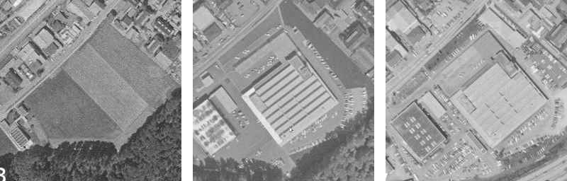
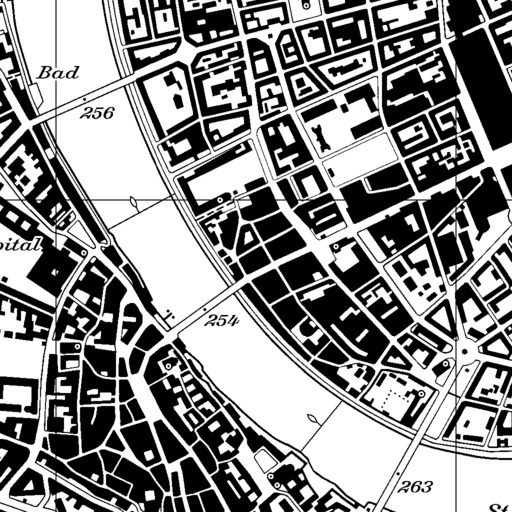
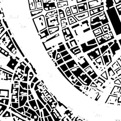
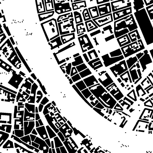
The following images give a geographical illustration of the selected areas through their most recent map:

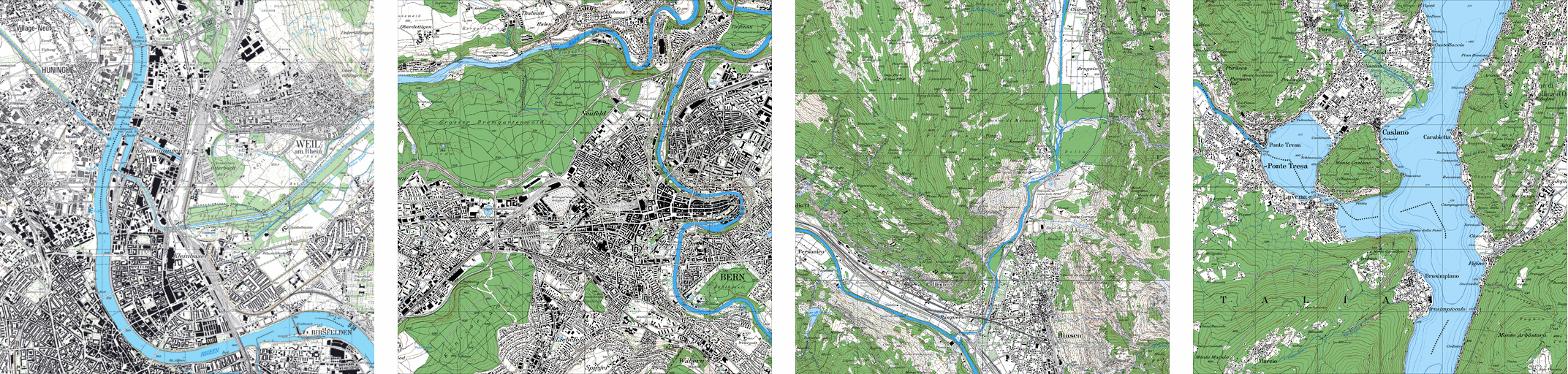
Illustration of the selected areas: Basel (2015), Bern (2010), Biasca (2012) and Caslano (2009)
Data: swisstopo

Basel was selected as it was one example of an area on which the building register was already well filled in terms of construction years. The four regions are 6km by 6km squared areas which allows up to twenty thousand buildings to be considered on a single one.

Federal Register of Buildings and Dwellings

The register of buildings is a formal database composed with entries, each of them representing a specific building. Each entry comes with a set of information related to the building they describe. In this project, a sub-set of these informations was considered:

• Federal identifier of the building (EGID)

• The position of the building, expressed in the EPGS:2056 (GKODE, GKODN)

• The building construction year, when available (GBAUJ)

• The surface of the building, when available, expressed in square metres (GAREA)

In addition, tests were conducted by considering the position of the entries of each building. In turned out rapidly that they were not useful in this research project as they were missing on a large fraction on the register and only providing a redundant information according to the position of the buildings.

The following table gives a summary of the availability of the construction year in the register according to the selected areas:

Area	Buildings	Available years	Missing fraction
Basel	17’088	16’584	3%
Bern	21’251	4’499	79%
Biasca	3’774	1’346	64%
Caslano	5’252	2’452	53%

One can see that the amount of missing construction year can be large depending on the considered area.

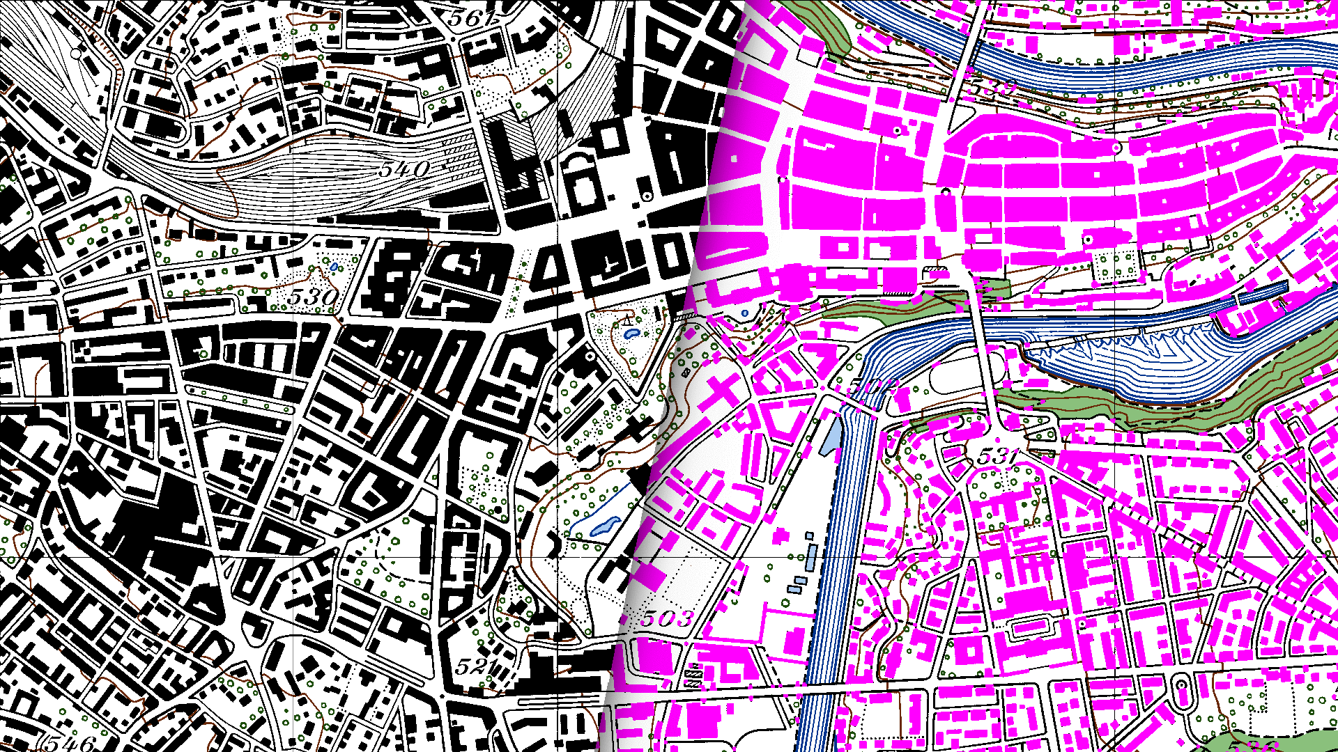
National Maps

On the side of the national maps, the dataset is more complex. In addition to the large number of available maps, variations of them can also be considered. Indeed, maps are made for different purposes and come with variations in their symbology to emphasise elements on which they focus. Moreover, for modern years, sets of vector data can also be considered in parallel to maps. Vector data are interesting as they allow to directly access the desired information, that is the footprint of the building without any processing required. The drawback of the vector data is their temporal coverage which is limited to the last ten to twenty years.

The following images give an illustration of the aspect of the available maps and vector datasets considering the example of the Bern area. Starting with the traditional maps:

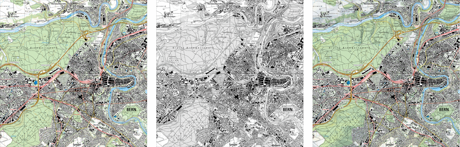
Available map variations: KOMB, KGRS and KREL - Data: swisstopo

and the more specific and vector ones:

Available map variations: SITU, GEB and DKM25-GEB (vector) - Data: swisstopo

In addition to the number of available variations and data types, they all come with their specific temporal coverage. In the case of this research project, we tried to go back in time as much as possible, simplifying the choice for the older maps. The question still remains for more modern times.

As we are mostly interesting in buildings, the availability of already extracted building layers, that can be either raster or vector data, is highly interesting. But the problem of data selection is complex in our case. Indeed, no matter the choice, on the older times, the only available maps have to be considered. In addition to building footprint access, the question of the continuity of the data as to be considered with care. More than building footprints, we are interested in the continuity of these footprints, in order to be able to safely assume the cycle of life of the tracker buildings.

This consideration led us to discover variation in methodologies depending on the considered set of data. Indeed, buildings are not shaped in the same way on traditional maps than they are in layer focusing on them. It follows that variation of the symbology, so do the shape of the building, appears between traditional maps and building layers (raster and vector). These variations can lead to shocks going from a map to the one preceding it in time. This can break the continuity of the building footprints along time, making them much more difficult to track safely.

This is the reason we choose to focus on the KOMB variation of the maps. These maps are very stable and covers the largest temporal ranges. The methodology was kept very similar along the years, making this dataset much more reliable to work with when the time dimension is considered. Only considering the KOMB variation of the maps also allows to ensure that all source data is treated the same in the processing pipeline, easing the assessment of the results.

In addition, the KOMB maps are dense in information and come with colorimetry of their symbology. This opens the possibility to more easily extract the information we need in this project, that are the building footprints. One exception was made concerning the KOMB maps: in their very latest version, the methodology changed, causing the symbology to be different with the older KOMB maps. In their latest version, texts are much more numerous and tend to cover a large amount of the buildings, making them invisible. For this reason, their latest version was dropped, slightly reducing the temporal coverage on the 2015-2020 period.

Selecting the KOMB variation allowed us to obtain the following temporal coverage for the four selected areas:

Area	Oldest map	Latest map	Mean separation
Basel	1955	2015	5.5 Years
Bern	1954	2010	5.6 Years
Biasca	1970	2012	6.0 Years
Caslano	1953	2009	6.2 Years

One can see that a large portion of the 20th century can be covered using the maps with a very good resolution of around five to six years between the maps.

Research Approaches

In this research project, the main focus was put on the national maps to extract the construction year of buildings as the maps are sources on which we can rely and assess the results. The only drawback of the maps is their limited temporal coverage, as they only start to be available in the 1950s.

This is the reason why another experimental approach was also added to address the cases of building being built before the 1950s. This secondary approach focused on a statistical methodology to verify to which extent it could be possible to assign a construction date even in the case no maps are available.

• National Maps: This main approach focuses on the national maps from which the construction year of a building is deduced from a temporal analysis of the maps. Each building is tracked until it disappears or change its shape on a given map allowing to deduce that the construction of the building was made in the gap separating the map and its successor one.

• Statistical Analysis: This method is based on the principle of spatial dependence and furthermore on concentric zones of urban development. This is technically an interpolator which deduces construction years based first on different searching radii for difference variances, second by splitting the data in quantiles and, finally, by a gaussian mixture model unsupervised learning technique to gather the final predictions.

The statistical analysis allows then to consider buildings that were detected on all maps, meaning their construction is older than the oldest available map, to assign them an estimation of their construction year, knowing they had to be older than the oldest map.

Research Approach: National Maps

In order to detect construction year of buildings, we need to be able to track them down on the maps across the temporal coverage. The RBD is providing the reference list of the building, each coming with a federal identifier (EGID) and a position. This position can then be used to track down the building on maps for its appearance or morphological change.

As the maps are already selected, as the research areas, this research approach can be summarised in the following way:

• Translating maps into binary images containing only building

• Extracting the RBD buildings related to the analysed area

• Detection procedure of the buildings on the maps

• Detection of the morphological variation of the buildings

• Assessment of the obtained results

The four first points are related to the development of the proof-of-concept. The last one concern a very sensitive and complicated question relative to the considered problem: how to analyse and assess the obtained results. This question was to most difficult question in this research, and finding a clear and reliable answer is mandatory before to develop anything. For this reason, it is considered in the first place.

Reliability of the Data

Assessing the results is essentially having a strong reference allowing to compare both in order to obtain a reliable characterisation of the success rate in the deduction of the construction years. This question leads to the discovery that this problem is much more complex that and can appear in the first place.

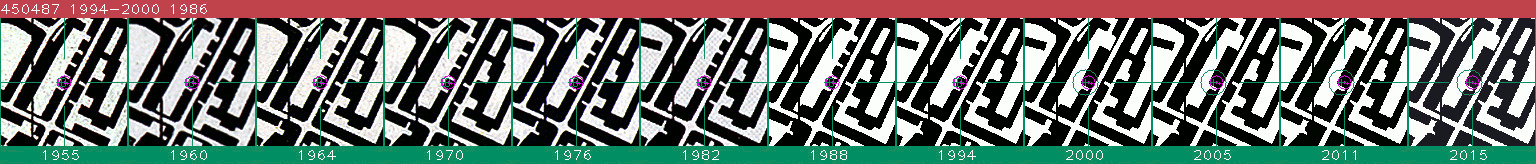
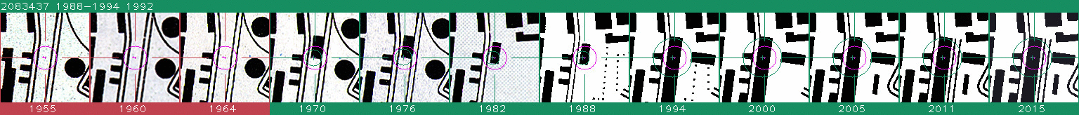
Indeed, we were warned by the Statistical Office that the RBD, considering the construction years it already gives, can be unreliable on some of its portions. This can be explained by the fact that collecting such information is a long and complicated administrative process. As an example, the following image gives an illustration of a building tracked on each of the available selected maps:

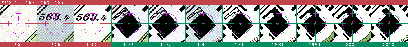
Temporal track of a selected building

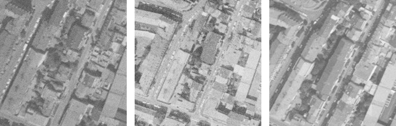
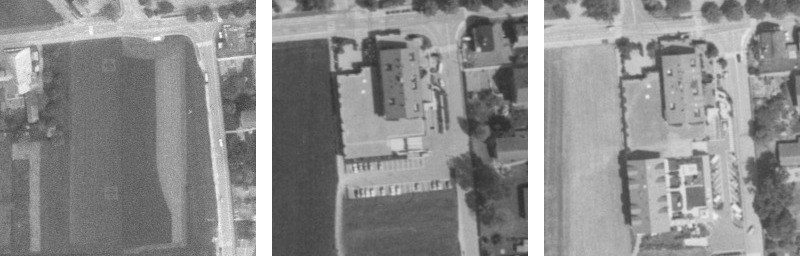
On this illustration, one can see two things: the RBD announce a construction year in 1985; the maps are clearly indicating something different, locating its construction year between 1963 and 1969. So both datasets are contradicting each other. In order to solve the contradiction, we manually searched for historical aerial images. The following images illustrate what was found:

Aerial view of the building situation: 1963, 1967 and 1987 - Data: swisstopo

One can clearly see that the maps seem to give the correct answer concerning the construction date of this specific building, the RBD being contradicted by two other sources. This illustrates the fact that the RBD can not be directly considered as a reliable reference to assess the results.

The same question applies for the maps. Even if it is believed that they are highly reliable, one has to be careful with such consideration. Indeed, looking at the following example:

Temporal track of a selected building

In this case, the RBD gives 1986 as the construction date of the pointed building. The maps are giving a construction year between 1994 and 2000. Again, the two datasets are contradicting each other. The same procedure was conducted to solve the contradiction:

Aerial view of the building situation: 1970, 1986 and 1988 - Data: swisstopo

Looking at the aerial images, it seems that the tracked building was there in 1988. One can see that the map in 1994 continue to represent the four old buildings instead on the new one. It's only in 2000 that the maps are correctly representing the new building. This shows that despite maps are a reliable source of geo-information, they can also be subjected to delay in their symbology.

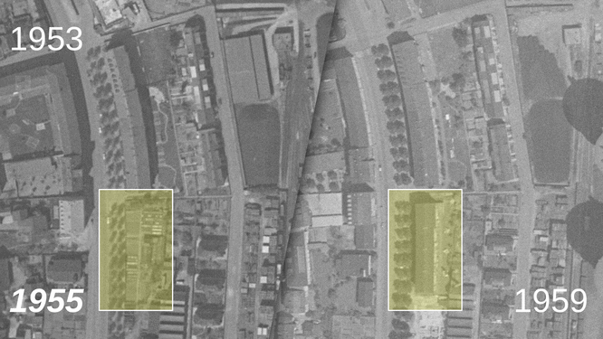
The maps also come with the problem of the consistency of the building footprint symbology. Looking at the following example:

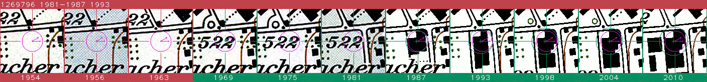
Temporal track of a selected building

one can see that the maps seem to indicate a strange evolution of the situation: a first building appears in 1987 and it is destroyed and replaced by a larger one in 1993. Then, this new large building seems to have been destroyed right after its construction to be replaced by a new one in 1998. Considering aerial images of the building situation:

Aerial image view of the building situation: 1981, 1987 and 1993 - Data: swisstopo

one can clearly see that a first building was constructed and completed by an extension between 1987 and 1993. This shows an illustration where the symbology of the building footprints can be subjected to variation than can be de-synchronised regarding the true situation.

Metric

In such context, neither the RBD or the national maps can be formally considered as a reference. It follows that we are left without a solution to assess our results, and more problematically, without any metric able to guide the developments of the proof-of-concept in the right direction.

To solve the situation, one hypothesis is made in this research project. Taking into account both the RBD and the national maps, one can observe that both are built using methodologies that are very different. On one hand, the RBD is built out of a complex administrative process, gathering the required information in a step by step process, going from communes to cantons, and finally to the Statistical Office. On the other hand, the national maps are built using regular aerial image campaigns conducted over the whole Switzerland. The process of establishing maps is quite old and can then be considered as well controlled and stable.

Both datasets are then made with methodologies that can be considered as fully independent from each other. This led us to the formulation of our hypothesis:

• Hypothesis: As the RBD and national maps are the results of independent methodologies, an error in one dataset is very unlikely to compensate an error in the other. In other words, if the RBD and the national maps agree on the construction year of a building, this information can be considered as a reliable reference, as it would be very unlikely to have two errors leading to such agreement.

One should remain careful with this hypothesis, despite it sounds reasonable. It would be very difficult to assess it as requiring to gather complex confirmation data that would have to be independent of the RBD, the national maps and the aerial images (as maps are based on them). This assumption is the only one made in this research project.

Accepting this assumption leads us to the possibility to establish a formal reference that can be used as a metric to assess the results and to guide the development of the proof-of-concept. But such reference has to be made with care, as the problem remains complex. To illustrate this complexity, the following figure gives a set representation of our problem:

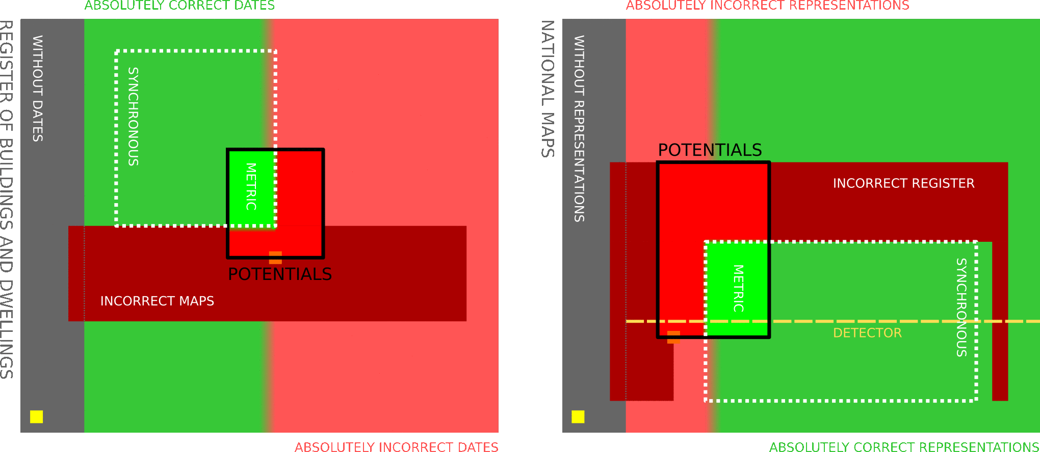
Set representation of the RBD completion problem

The two rectangles represent the set of buildings for a considered area. On the left, one can see the building set from the RBD point of view. The grey area shows the building without the information of their construction year. Its complementary set is split in two sub-sets that are the buildings having a construction year that is absolutely correct and absolutely incorrect (the limit between both is subject to a bit of interpretation, as the construction year is not a strong concept). If a reference can be extracted, it should be in the green sub-set. The problem is that we have no way of knowing which building are in which sub-set. So the national maps were considered to define another sub-set: the synchronous sub-set where both RBD and national maps agree.

To build the metric, the RBD sub-set of buildings coming with the information of the construction year is randomly sub-sampled to extract a representative sub-set: the potentials. This sub-set of potentials is then manually analysed to separate the building on which both datasets agree and to reject the other. At the end of the process, the metric sub-set is obtained and should remain representative.

On the right of the set representation is the view of the buildings set through the national maps. One can see that the same sub-set appears but it replaces the construction years by the representation of the building on the maps. The grey part is then representing the building that are not represented on the maps because of their size or because they can be hidden by the symbology for example. The difference is that the maps do not give access to the construction years directly, but they are read from the maps through our developed detector. The detector having a success rate, it cuts the whole set of sub-sets in half, which is exactly what we need for out metric. If the metric sub-set remains representative, the success rate of the detector evaluated on it should generalise to the whole represented buildings.

This set representation demonstrates that the problem is very complex and has to be handled with care. Considering only the six most important sub-set and considering construction year are extracted by the detector from the maps, it means that up to 72 specific case can apply on each building randomly selected.

To perform the manual selection, a random selection of potential buildings was made on the RBD set of buildings coming with a construction year. The following table summarises the selection and manual validation:

Area	Potentials	Metric
Basel	450 EGIDs	209 EGIDs
Bern	450 EGIDs	180 EGIDs
Biasca	336 EGIDs	209 EGIDs
Caslano	450 EGIDs	272 EGIDs

The previous table gives the result of the second manual validation. Indeed, two manual validation sessions were made, with several weeks in-between, to check the validation process and how it evolved with the increase of the view of the problem.

Three main critics can then be addressed to the metric: the first one is that establishing validation criterion is not simple as the number of cases in which buildings can fall is very high. Understanding the problem takes time and requires to see a lot of these cases. It then follows that the second validation session was more stable and rigorous than the first one.

The second critic that can be made on our metric is the selection bias. As the process is made by a human, it is affected by its way of applying the criterion and more specifically on by its severity on their application. Considering the whole potentials sub-set, one can conclude that a few buildings could be rejected and validated depending on the person doing the selection.

The last critic concerns specific cases for which the asynchronous criterion to reject them is weak. Indeed, for some buildings, the situation is very unclear in the way the RBD and the maps give information that can not be understood. This is the case for example when the building is not represented on the map. This can be the position in the RBD or the lack of information on the maps that lead to such an unclear situation. These cases are then rejected, but without being fully sure of the asynchronous aspect regarding the maps and the RBD.

Methodology

With a reliable metric, results can be assessed and the development of the proof-of-concept can be properly guided. As mentioned above, the proof-of-concept can be split in four major steps that are the processing of the maps, the extraction of the RBD buildings, detection of the building on the maps and detection in morphological changes.

National Maps Processing

In order to perform the detection of building on the maps, a reliable methodology is required. Indeed, one could perform the detection directly on the source maps but this would lead to a complicated process. Indeed, maps are mostly the result of the digitisation of paper maps creating a large number of artefacts on the digital images. This would lead to an unreliable way of detecting building as a complicated decision process would have to be implemented each time a RBD position is checked on each map.

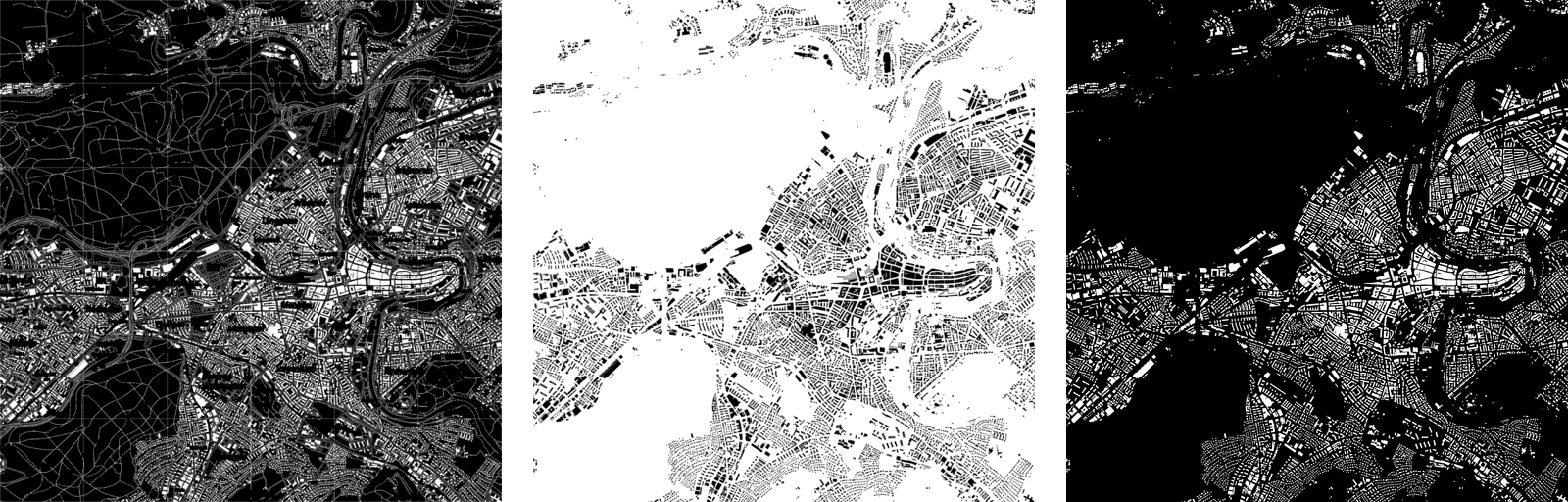
A map processing step was then introduced in the first place allowing to translate the color digitised images into reliable binary images on which building detection can be made safely and easily. The goal of this process is then to create a binary version of each map with black pixels indicating the building presence. A method of extracting buildings on maps was then designed.

Considering the following example of a map cropped according to a defined geographical area (Basel):

 
Example of a considered map: Basel in 2005 and closer view - Data: swisstopo

The first step of the map processing methodology is to correct and standardise the exposure of the digitised maps. Indeed, as maps mostly result of a digitisation process, they are subjected to exposure variation due to the digitisation process. A simple standardisation is then applied.

The next step consists in black pixel extraction. Each pixel of the input map is tested to determine whether or not it can be considered as black using specific thresholds. As the building are drawn in black, extracting black pixels is a first way of separating the buildings from the rest of the symbology. The following result is obtained:

 
Result of the black extraction process

As one can see on the result of the black extraction process, the buildings are still highly connected to other symbological elements and to each others in some cases. Having the building footprints well separated and well defined is an important point for subsequent processes responsible of construction years deduction. To achieve it, two steps are added. The first one uses a variation of the Conway game of life [5] to implement a morphological operator able to disconnect pixel groups. The following image gives the results of this separation process along with the previous black extraction result on which it is based:

 
Result of the morphological operator (right) compare to the previous black extraction (left)

As the morphological operator provides the desired result, it also shrinks the footprint of the elements. It allows to eliminate a lot of structures that are not buildings, but it also reduces the footprint of the buildings themselves, which can increase the amount of work to perform by the subsequent processes to properly detect a building. To solve this issue and to obtain building footprints that are as close as possible to the original map, a controlled re-growing step is added. It uses a region threshold and the black extraction result to re-grow the buildings without going any further of their original definition. The following images give a view of the final result along with the original map:

 
Final result of the building footprints extraction (right) compared to the original map

As the Conway morphological operator is not able to get rid of all the non-building elements, such as large and bold texts, the re-growing final step also thickening them along with the building footprints. Nevertheless, the obtained binary image is able to keep most of the building footprint intact while eliminating most of the other element of the map as illustrated on the following image:

Extracted building footprints, in pink, superimposed on the Bern map

The obtained binary images are then used for both detection of building and detection of morphological changes as the building are easy to access and to analyse on such representation.

Building Extraction from RBD

In the case of limited geographical areas as in this research project, extracting the relevant buildings from the RBD was straightforward. Indeed, the RBD is a simple DSV database that is very easy to understand and to process. The four areas were packed into a single DSV file and the relevant building were selected through a very simple geographical filtering. Each area being defined by a simple geographical square, selecting the buildings was only a question of checking if their position was in the square or not.

Building Detection Process

Based on the computed binary images, each area can be temporally covered with maps on which building can be detected. Thanks to the processed maps, this detection is made easily, as it was reduced to detect black pixels in a small area around the position of the building provided in the RBD. For each building in the RBD, its detection on each temporal version of the map is made to create a presence table of the building. Such table is simply a Boolean value indicating whether a building was there or not according to the position provided in the RBD.

The following images give an illustration of the building detection process on a given temporal version of a selected map:

 
Detection overlay superimposed on its original map (left) and on its binary counterpart (right)

One can see that for each building and for each temporal version of the map, the decision of a building presence can be made. At the end of this process, each building is associated to a list of presence at each year corresponding to an available map.

Morphological Change Detection

Detecting the presence of a building on each temporal version of the map is a first step but is not enough to determine whether or not it is the desired building. Indeed, a building can be replaced by another along the time dimension without creating a discontinuity in the presence timeline. This would lead to misinterpret the presence of building with another one, leading the construction year to be deduced too far in time. This can be illustrated by the following example:

Example of building being replaced by another one without introducing a gap in the presence table

In case the detection of the presence of the building is not enough to correctly deduce a construction year, a morphological criterion is added. Many different methodologies have been tried in this project, going from signature to various quantities deduce out of the footprint of the building. The most simple and most reliable way was to focus on the pixel count of the building footprint, which corresponds to its surface in geographical terms.

A morphological change is considered as the surface of the building footprint changes up to a given threshold along the building presence timeline. In such a case, the presence timeline is broken at the position of the morphological change, interpreting it in the same way as a formal appearance of a building.

Introducing such criteria allowed to significantly improve our results, especially in the case of urban centers. Indeed, in modern cities, large number of new buildings were built just after a previous building was being destroyed due to the lack of spaces left for new constructions.

Results

The developed proof-of-concept is applied on the four selected areas to deduce construction year for each building appearing in the RBD. With the defined metric, it is possible to assess the result in a reliable manner. Nevertheless, assessing the results with clear representations is not straightforward. In this research project, two representations were chosen:

• Histogram of the success rate: For this representation, the building of the metric are assigned to temporal bins of ten years in size and the success rate of the construction year is computed for each bins.

• Distance and pseudo-distance distribution: As the previous representation only gives access to a binary view of the results, a distance representation is added to understand to which extent mistakes are made on the deduction of a construction year. For buildings detected between two maps, the temporal middle is assumed as the guessed construction year, allowing to compute a formal distance with its reference. In case a building is detected before or beyond the map range, a pseudo-distance of zero is assigned in case the result is correct according to the reference. Otherwise, the deduced year (that is necessarily between two maps) is compared to its reference extremal map date to obtain an error pseudo-distance.

In addition to the manually defined metric, the full RBD metric is also considered. As the construction years provided in the RBD have to be considered with care, as part of them are incorrect, comparing the results obtained the full RBD metric and the metric we manually defined opens the important question of the synchronisation between the maps and the RBD, viewed from the construction perspective.

Results: Basel Area

The following figures give the Basel area result using the histogram representation. The left plot uses the full RBD metric while the right one uses the manually validated one:

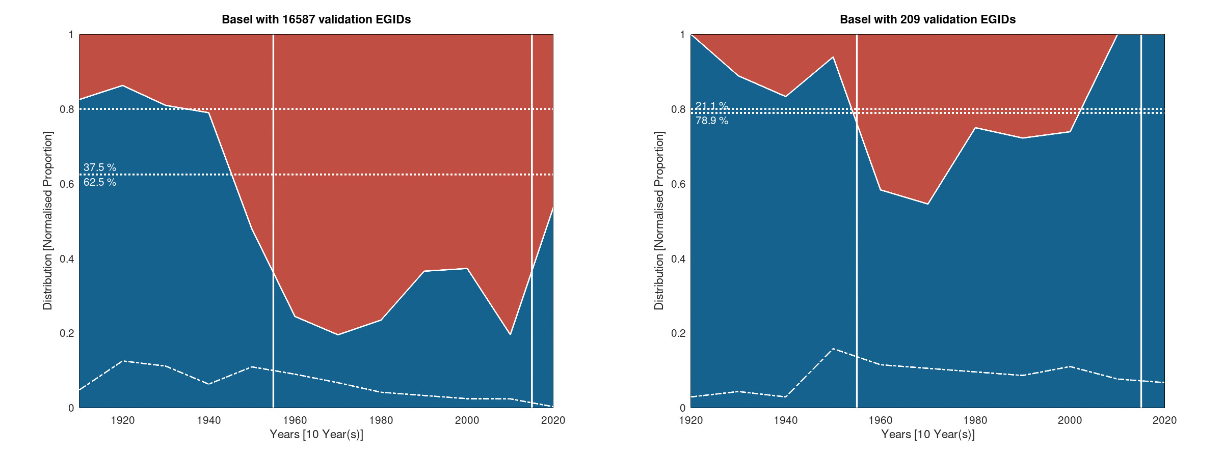
Histogram of the success rate - Ten years bins

One can see one obvious element that is the result provided by the full RBD metric (left) and the manually validated metric (right) are different. This is a clear sign that the RBD and the maps are de-synchronised on a large fraction of the building set of Basel. The other element that can be seen on the right plot is that the deduction of the construction year are more challenging where maps are available. Indeed on the temporal range covered by the maps (vertical white lines), the results drops from the overall results to 50-60% on some of the histogram bins.

The following figures show the distance and pseudo-distance distribution of the error made on the deduced construction year according to the chosen metric:

Distance (red and blue) and pseudo-distance (red) of the error on the construction years

The same differences as previously observed between the two metrics can also be seen here. Another important observation is that the distribution seems mostly symmetrical. This indicates that no clear deduction bias can be observed in the results provided by the proof-of-concept.

Results: Bern Area

The following figures give the histogram view of the results obtained on the Bern area:

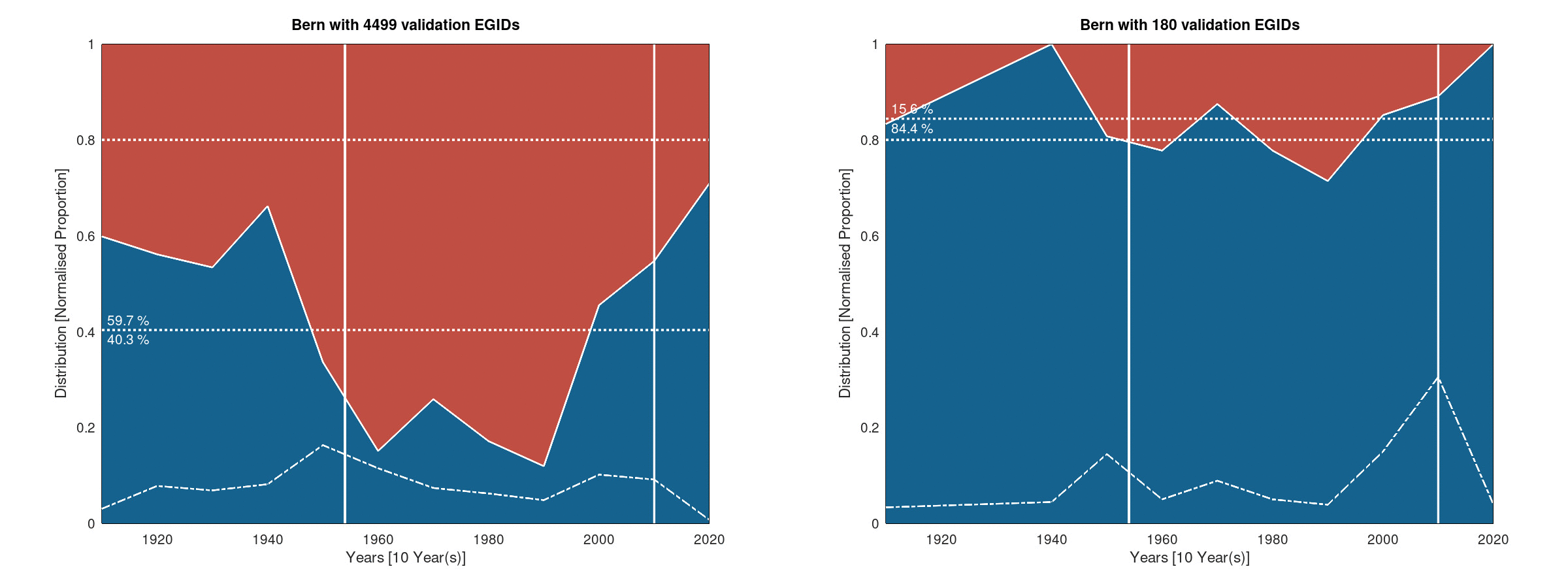
Histogram of the success rate - Ten years bins

One can observe that the results are similar to the result of Basel whilst being a bit better. In addition, one can clearly see that the difference between the full RBD metric and the manually validated metric huge here. This is probably the sign that the RBD is mostly incorrect in the case of Bern.

The following figures show the distance distributions for the case of Bern:

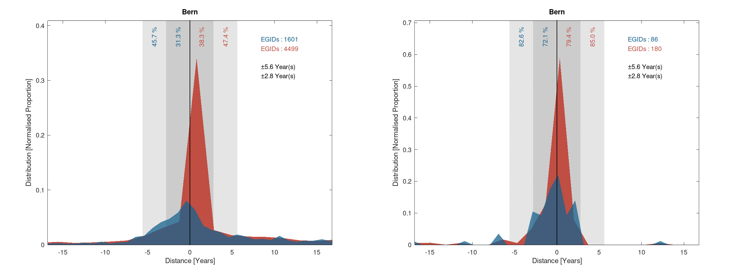
Distance (red and blue) and pseudo-distance (red) of the error on the construction years

Again, the distribution of the error on the deduced construction year is symmetrical in the case of Bern.

Results: Biasca Area

The following figures give the histogram view of the success rate for the case of Biasca:

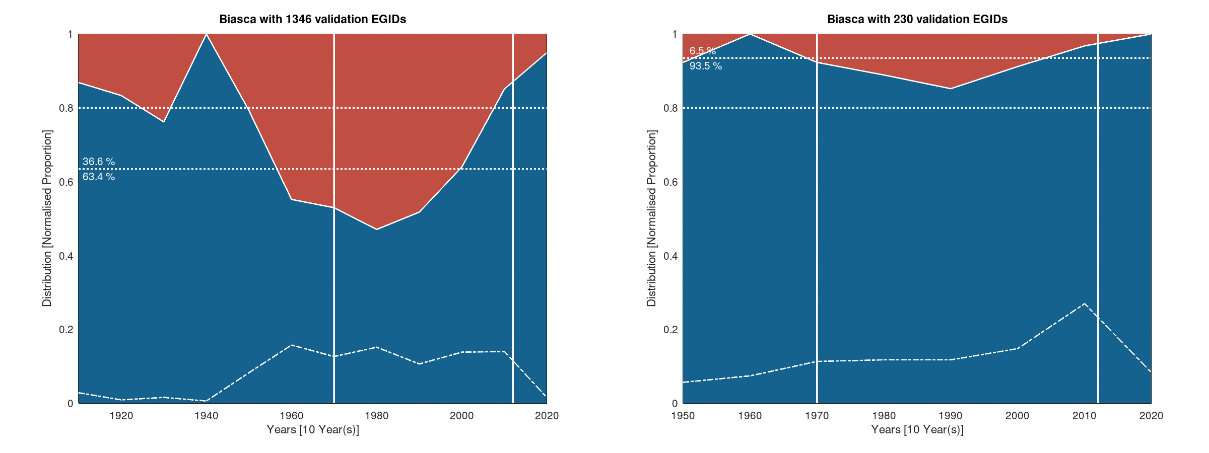
Histogram of the success rate - Ten years bins

In this case, the results are much better according to the manually validated metric. This can be explained by the fact that Biasca is a rural/mountainous area in which growing of the urban areas are much simpler as buildings once built tend to remain unchanged, limiting the difficulty to deduce a reliable construction year.

The following figures show the distance distribution for Biasca:

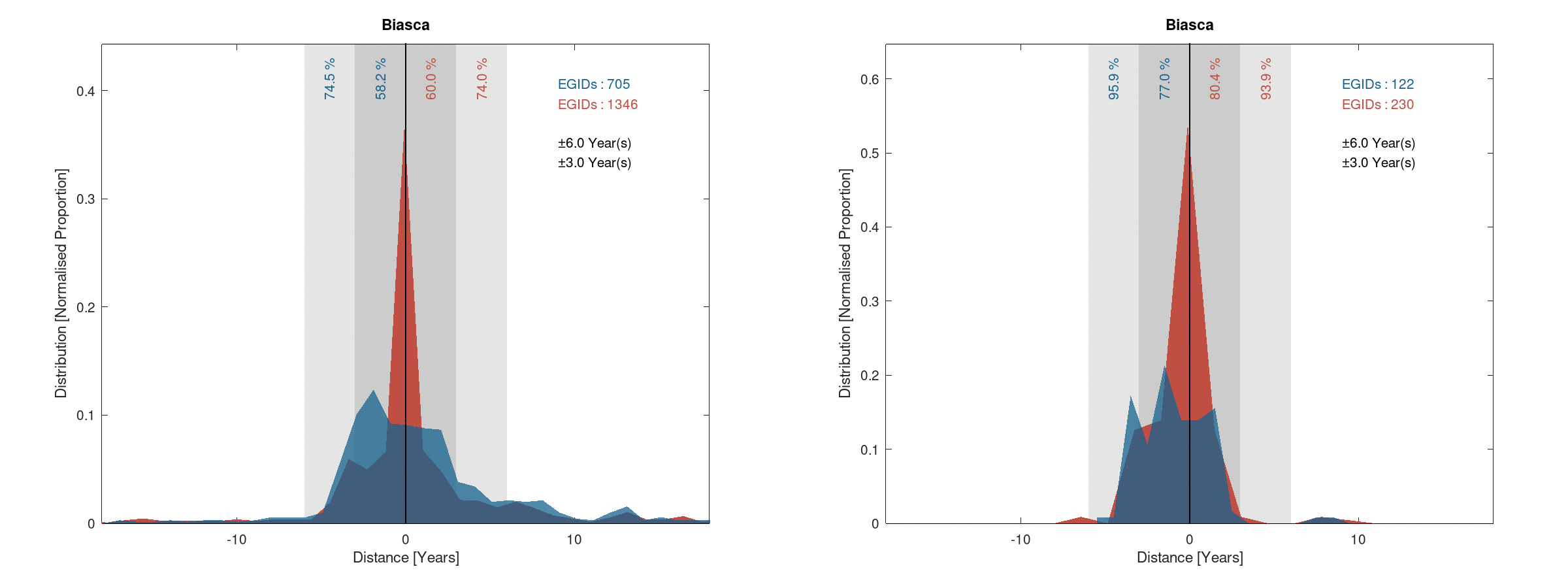
Distance (red and blue) and pseudo-distance (red) of the error on the construction years

This confirms the results seen on the histogram figure and shows that the results are very good on such areas.

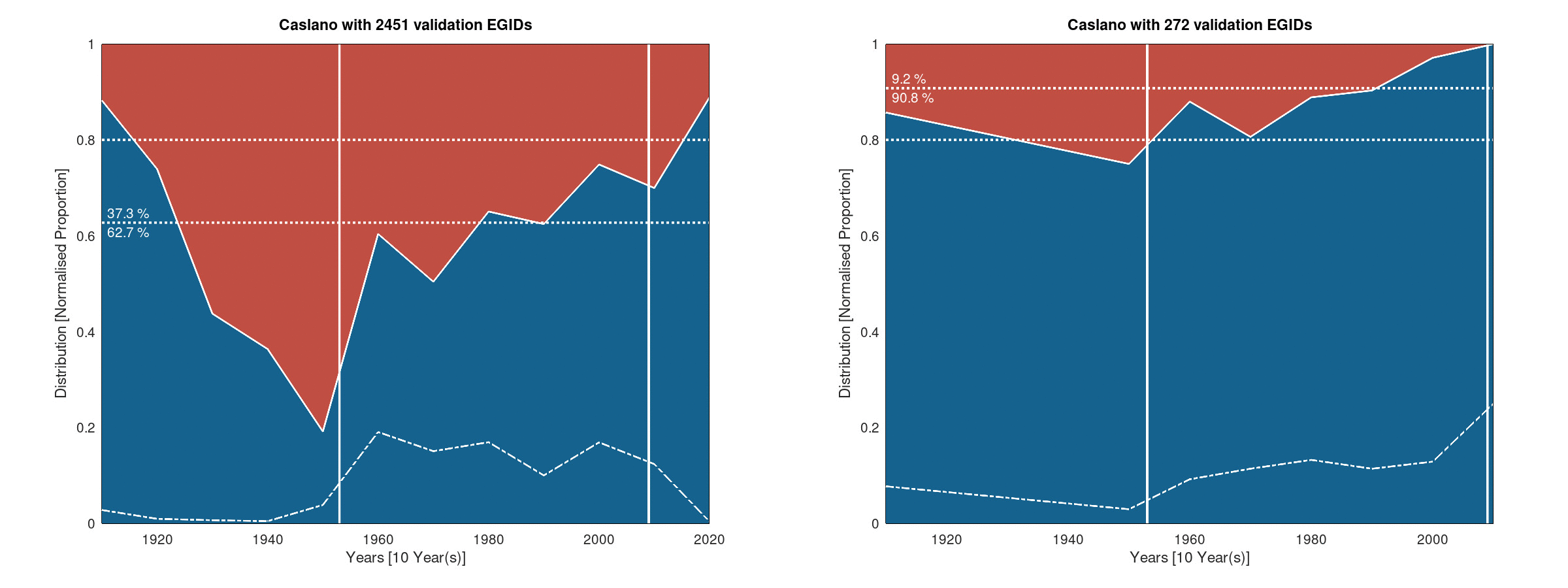
Results: Caslano Area

Finally, the following figures show the histogram view of the success rate of the proof-of-concept on the case of Caslano:

Histogram of the success rate - Ten years bins

The same consideration applies as for the Biasca case. The results are very good as part of the Caslano area can be considered as rural or at least peri-urban. The results are a bit less good than in the Biasca case, drawing the picture that urban centres are more difficult to infer than rural areas.

The following figures show the error distribution for Caslano:

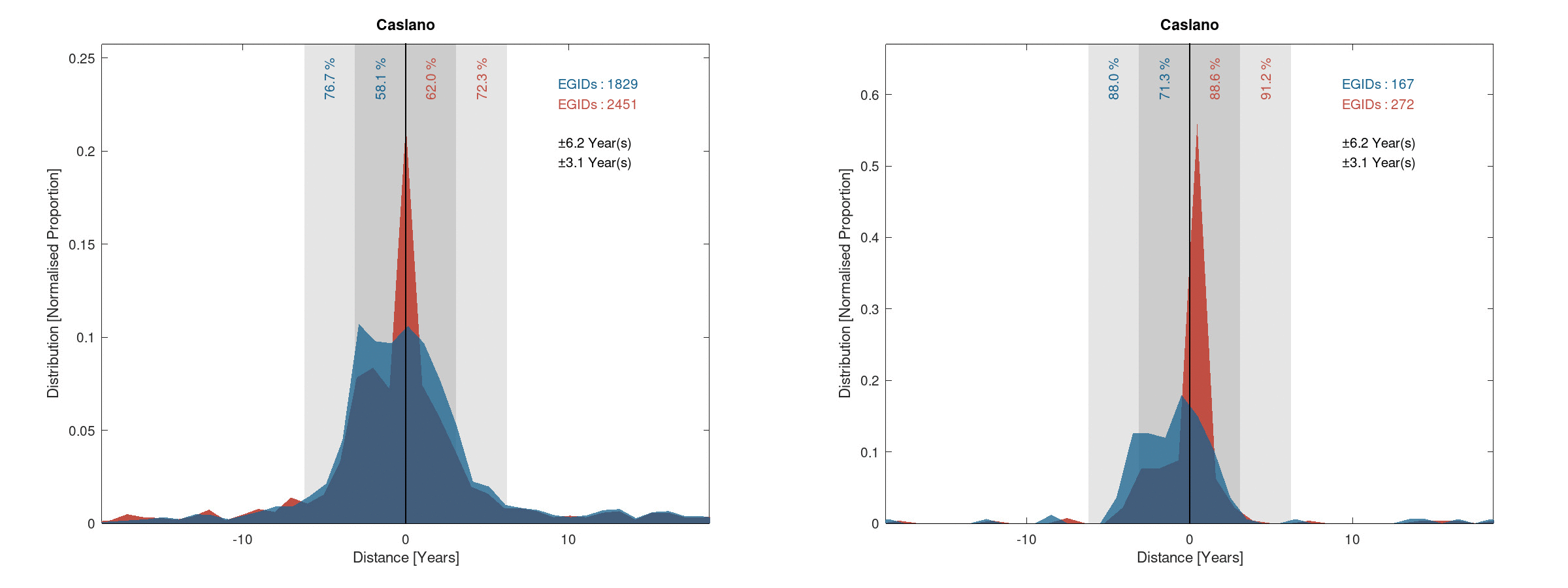
Distance (red and blue) and pseudo-distance (red) of the error on the construction years

Results: Synthesis

In order to synthesise the previous results, that were a bit dense due to the consideration of two representations and two metrics, the following summary is given:

• Basel: 78.0% of sucess rate and 80.4% of building correctly placed within ±5.5 years

• Bern: 84.4% of sucess rate and 85.0% of building correctly placed within ±5.6 years

• Biasca: 93.5% of sucess rate and 93.9% of building correctly placed within ±6.0 years

• Caslano: 90.8% of sucess rate and 91.2% of building correctly placed within ±6.2 years

These results only consider the manually validated metric for all of the four areas. By weighting each area with their amount of buildings, one can deduce the following numbers:

• Switzerland: 83.9% of success rate and 84.7% of building correctly place within ±5.8 years

These last numbers can be considered as a reasonable extrapolation of the proof-of-concept performance on the overall Switzerland.

Conclusion

As a main conclusion to the national maps approach, one can consider the results as good. It was possible to develop a proof-of-concept and to apply it on selected and representative areas of Switzerland.

In this approach, it turns out that developing the proof-of-concept was the easy part. Indeed, finding a metric and demonstrating its representativeness and reliability was much more complicated. Indeed, as the two datasets can not be considered as fully reliable in the first place, a strategy had to be defined in order to be able to demonstrate that the chosen metric was able to assess our result in the way expected by the Statistical Office.

In addition, the metric only required one additional hypothesis on top of the two datasets. This hypothesis, consisting in assuming that the synchronous sub-set was a quasi-sub-set of the absolutely correct construction years, can be assumed to be reasonable. Nevertheless it is important to emphasise that it was necessary to make it, leading us to remains critic and careful whilst reading the results given by our metric.

The developed proof-of-concept was developed in C++, leading to an efficient code able to be used for the whole processing of Switzerland without the necessity to deeply modify it.

Research Approach: Statistical

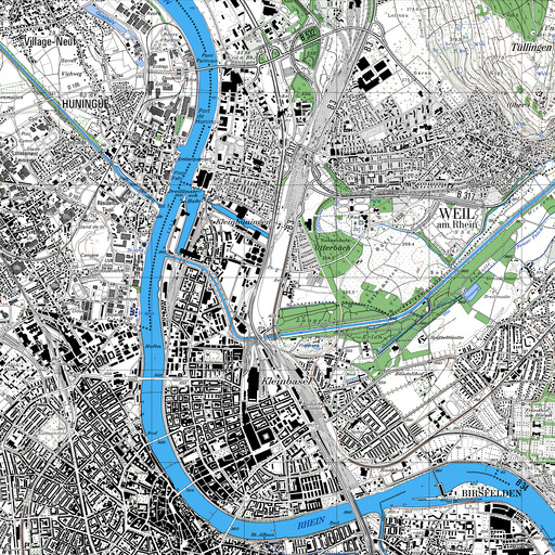
As the availability of the topographic/national maps does not reach the integrity of all building's year of construction in the registry, an add-on was developed to infer this information, whenever there was this need for extrapolation. Usually, the maps availability reaches the 1950s, whilst in some cities the minimum year of construction can be in the order of the 12th century, e.g. The core of this statistical model is based on the Concentric Zones Model (Park and Burgess, 1925)[6] extended to the idea of the growth of the city from the a centre (Central Business District - CBD) to all inner areas. The concept behind this statistical approach can be seen below using the example of a crop of Basel city:

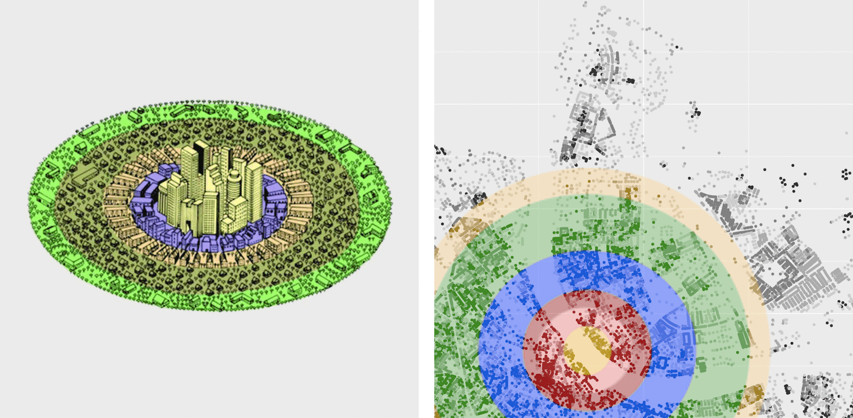
Illustration of the Burgess concentric zone model

Although it is well known the limits of this model, which are strongly described in other famous urban models such as from Hoyt (1939)[7] and Harris and Ullman (1945)[8]. In general those critics refer to the simplicity of the model, which is considered and compensated for this application, especially by the fact that the main prediction target are older buildings that are assumed to follow the concentric zones pattern, differently than newer ones (Duncan et al., 1962)[9]. Commonly this is the pattern seen in many cities, hence older buildings were built in these circular patterns to some point in time when reconstructions and reforms are almost randomly placed in spatial and temporal terms. Moreover processes like gentrification are shown to be dispersed and quite recent (Rérat et al, 2010)[10].

In summary, a first predictor is built on the basis that data present a spatial dependence, as in many geostatistical models (Kanevski and Maignan, 2004[11]; Diggle and Ribeiro, 2007[12]; Montero and Mateu, 2015[13]). This way we are assuming that closer buildings are more related to distant buildings (Tobler, 1970[14]) in terms of year of construction and ergo the time dimension is being interpolated based on the principles of spatial models. We are here also demonstrating how those two dimensions interact. After that concentric zones are embedded through the use of quantiles, which values will be using in a probabilistic unsupervised learning technique. Finally, the predicted years are computed from the clusters generated.

Metric

Similar to the detection situation, generating a validation dataset was an especially challenging task. First of all, the dates in the RBD database could not be trusted in their integrity and the topographic maps used did not reach this time frame. In order to ascertain the construction year in the database, aerial images from swisstopo (Swiss Federal Office of Topography) were consulted and this way buildings were manually selected to compound a validation dataset.

References extraction from aerial images manual analysis

One of the problems related to this approach was the fact that a gap between the surveys necessary for the images exists. This way it is not able to state with precision the construction date. These gaps between surveys were approximately in the range of 5 years, although in Basel, for some areas, it reached 20 years. An example of this methodology to create a trustworthy validation set can be seen below. In the left-hand side one can see the year of the first image survey (up) and the year registered in the RBD (down) and in the right-hand side, one can see the year of the next image survey in the same temporal resolution.

Methodology

First of all, a prior searching radius is defined as half of the largest distance (between random variables). For every prediction location, the variance between all points in the prior searching radius will be used to create a posterior searching radius. This way, the higher the variance, the smaller the searching radius, as we tend to trust data less. This is mainly based on the principle of spatial dependence used in many geostatistical interpolators. The exception to this rule is for variances that are higher than 2 x the mean distance between points. In this case, the searching radius increases again in order to avoid clusters of very old houses that during tests caused underestimation. The figure below demonstrates the logic being the creation of searching radii.

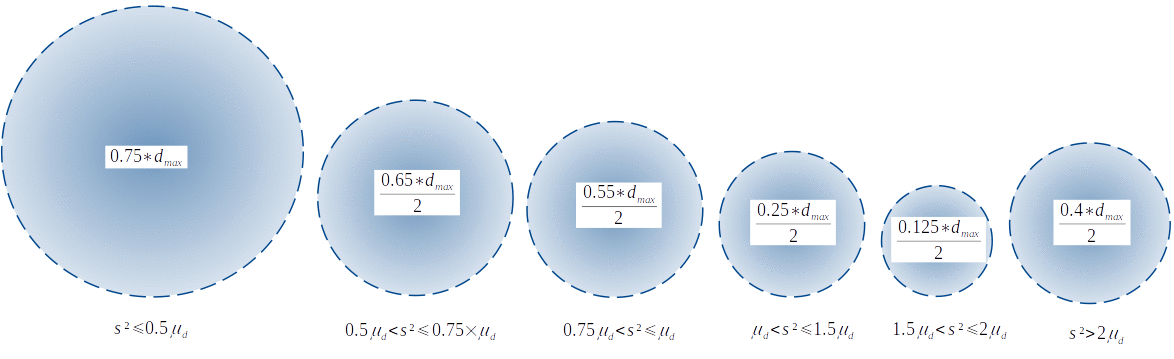
Searching radii computation process

being d the distance between points, μ the mean and s² the variance of random variable values within the prior searching radius.

It is important to mention that in case of very large number of missing data, if the searching radius does not find enough information, the posterior mean will be the same as the prior mean, possibly causing over/underestimation in those areas.

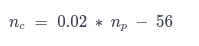
This first procedure is used to fill the gaps in the entry database so clustering can be computed. The next step is then splitting the data in 10 quantiles, what could give the idea of concentric growth zones, inspired, in Burgess Model (1925)[7]. Every point in the database will then assume the value of its quantile. It is also possible to ignore this step and pass to clustering directly, what can be useful in two situations, if a more general purpose is intended or if the concentric zones pattern is not observed in the study area. As default, this step is used, which will be followed by an unsupervised learning technique. A gaussian mixture model, which does not only segments data into clusters, but indicates the probability of each point belonging to every cluster is then performed. The number of components computed is a linear function to the total number of points being used, including the ones that previously had gaps. The function to find the number of components is the following:

being np the number of components/clusters, and nc the total number of points used. The number of clusters shall usually be very large compared to a standard clustering exercise. To avoid this, this value is being divided by ten, but the number of clusters will never be smaller than five. An example of clustering performed by the embedded gaussian mixture model can be seen below:

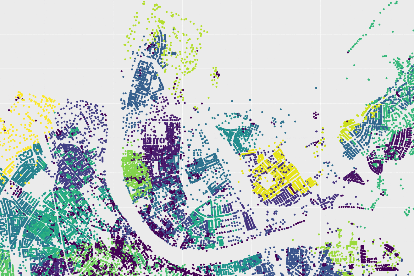
Example of clustering process on the Basel area

Hence the matrix of probabilities of every point belonging to each cluster (λ - what can be considered a matrix of weights) is multiplied by the mean of each cluster ( 1 x nc matrix mc), forming the A matrix:

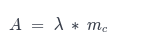
or in matrices:

Finally, the predictions can then be made using the sum of each row in the A matrix.

It is important to state that the same crops (study areas) were used for this test. Although Caslano was not used in this case, as it possesses too few houses with a construction date below the oldest map available. Using the metric above explained a hold out cross-validation was performed, this way a group of points was only used for validation and not for training. After that, the RMSE (Root Mean Squared Error) was calculated using the difference between the date in the RBD database and the predicted one. This RMSE was also extrapolated to the whole Switzerland, so one could have a notion of what the overall error could be, using the following equation (for the expected error):

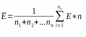
where E is the error and n the number of buildings in each region.

In addition to the RMSE, the 95th percentile was computed for every study area and using all combined as well. Hence, one could discuss the spread and predictability of errors.

Results

The first case analysed was Basel, where the final RMSE was 9.78 years. The density plot below demonstrates the distribution of errors in Basel, considering the difference between the year of construction in the RBD database and the predicted one.

Distribution of error on construction year extrapolation

Among the evaluated cases, Basel presented a strong visible spatial dependence, and it was also the case which the largest estimated proportion of houses with construction years older than (1955) the oldest map (11336 or approximately 66% of buildings). Based on the validation dataset only, there was an overall trend of underestimation and the 95th percentile reached was 20 years, showing a not so spread and flat distribution of errors.

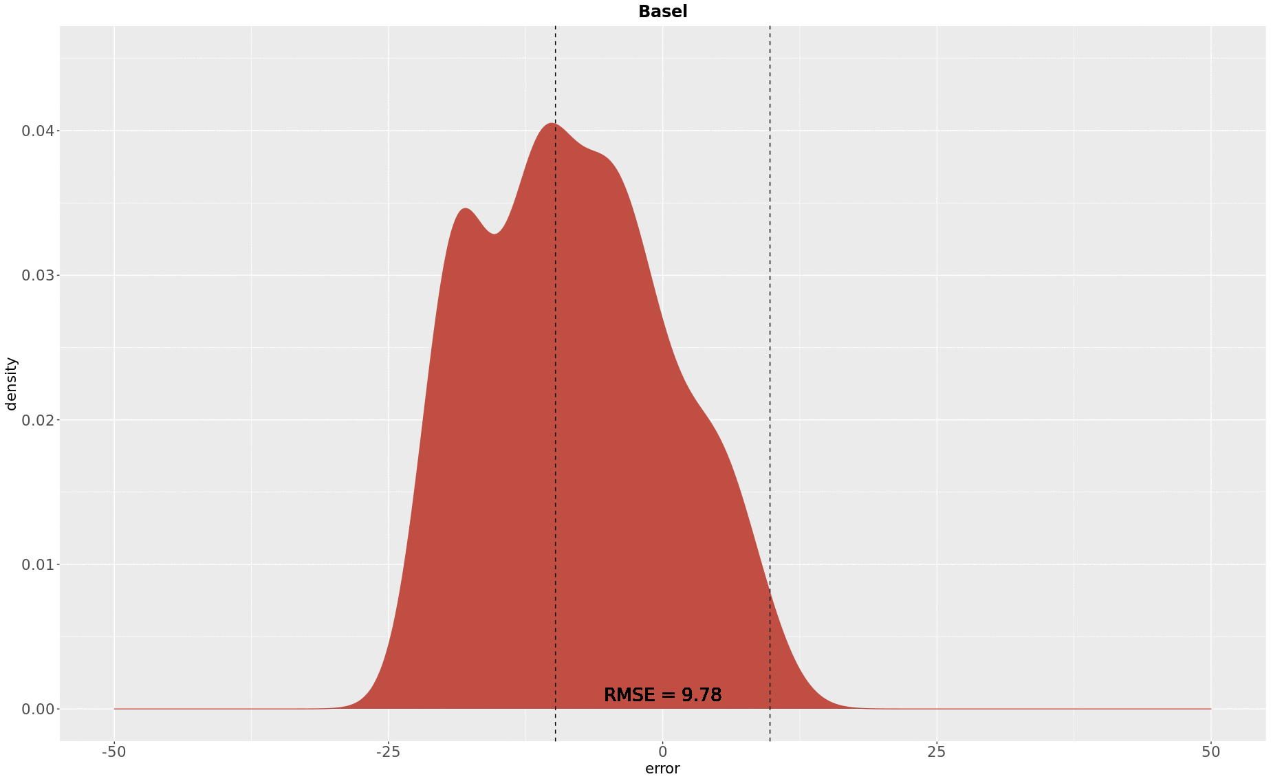
Bern was the second case evaluated, and it demonstrated to be an atypical case. This starts from the fact that a big portion of the dates seemed incongruent with reality, based on the aerial images observed and as seen in the previous detection approach. Not only that, but almost 80% of the buildings in Bern had missing data to what refers to the year of construction. This is especially complicated as the statistical method here presented is in essence an interpolator (intYEARpolator). Basically, as in any inference problem, data that is known is used to fill unknown data, therefore a reasonable split among known and unknown inputs is expected, as well as a considerable confidence on data. In the other hand, an estimated number of 1079 (approximately 27% of the buildings) buildings was probably older than the oldest map available (1954) in Bern crop. Therefore, in one way liability was lower in this case, but the number of prediction points was smaller too. The following figure displays the density of errors in Bern, where an RMSE of 20.64 years was computed.

Distribution of error on construction year extrapolation

There was an overall trend for overestimation, though there was still enough lack of spread in errors, especially if one considers the 95th percentile of 42.

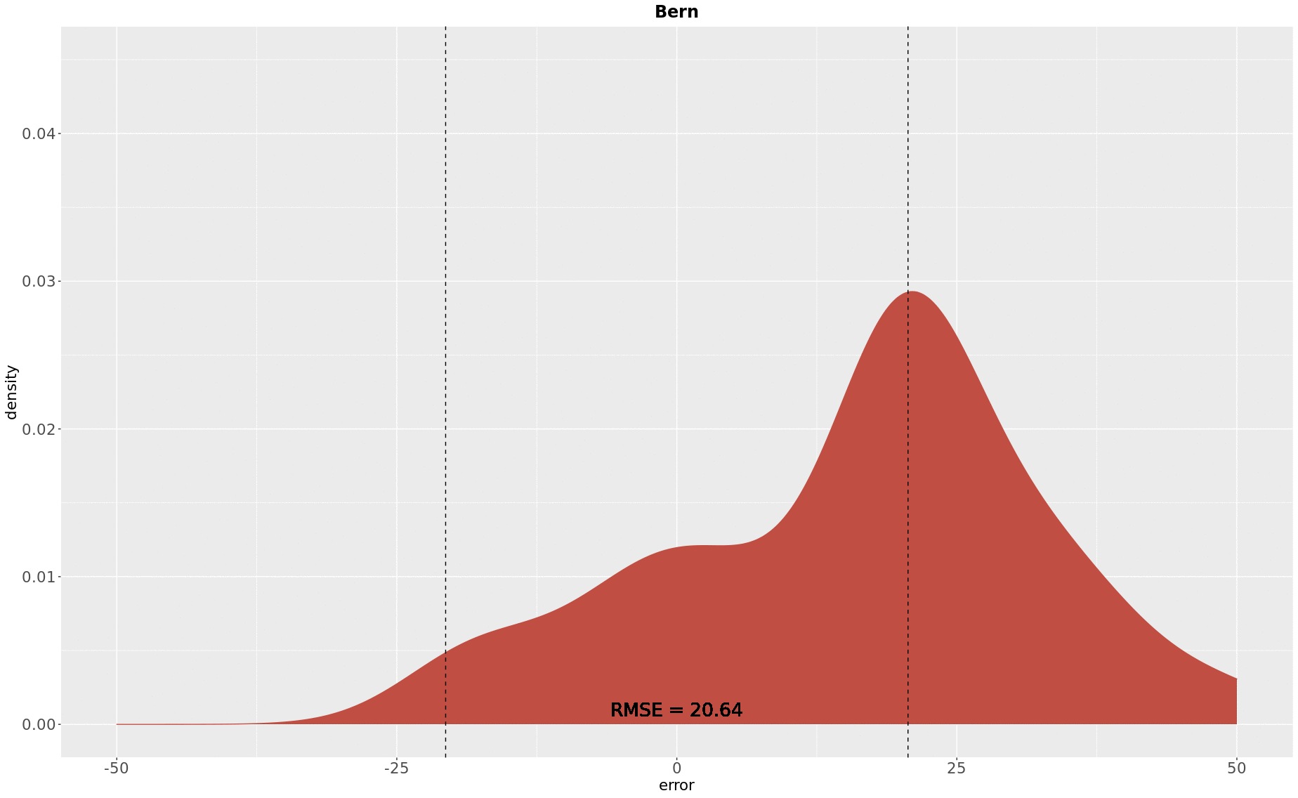
Finally, the crop on Biasca was evaluated. The computed RMSE was of 13.13 years, which is closer to the Basel case and the 95th percentile was 17 years, this way presenting the least spread error distribution. In Biasca an estimated 1007 (32%) buildings were found, which is not much more than the proportion in Bern, but Biasca older topographic map used was from 1970, making of it an especially interesting case. The density plot below demonstrates the concentrated error case of Biasca:

Distribution of error on construction year extrapolation

Once the RMSE was computed for the three regions, it was extrapolated to the whole Switzerland by making consideration the size of each dataset:

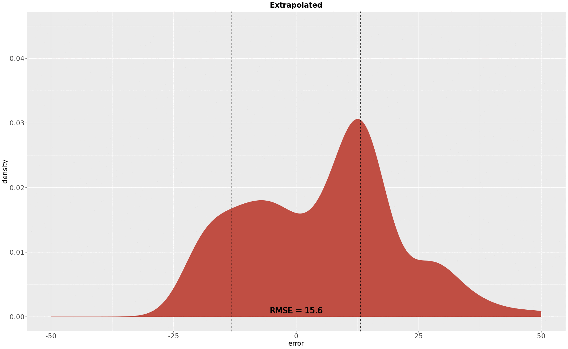
Extrapolation of the error distribution on the whole Switzerland

The expected extrapolated error calculated was 15.6 years and the 95th percentile was then 31 years.

Conclusion

This add-on allows extrapolating the predictions to beyond the range of the topographical maps. Its predictions are limited, but the accuracy reached can be considered reasonable, once there is a considerable lack of information in this prediction range. Nor the dates in the RBD, nor the topographic maps can be fully trusted, ergo 15.6 years of error for the older buildings is acceptable, especially by considering the relative lack of spread in errors distribution. If a suggestion for improvement were to be given, a method for smoothing the intYEARpolator predictions could be interesting. This would possibly shift the distribution of the error into closer to a gaussian with mean zero. The dangerous found when searching for such an approach is that the year of construction of buildings does not seem to present a smooth surface, despite the spatial dependence. Hence, if this were to be considered, a balance between smoothing and variability would need to found.

We also demonstrated a completely different perspective on how the spatial and temporal dimensions can be joined as the random variable predicted through spatial methodology was actually time. Therefore a strong demonstration of the importance of time in spatially related models and approaches was also given. The code for the intYEARpolator was developed in Python and it runs smoothly even with this quite big proportion of data. The singular case it can be quite time-demanding is in the case of high proportion of prediction points (missing values). It should also be reproducible to the whole Switzerland with no need for modification. A conditional argument is the use of concentric zones, that can be excluded in case of a total different pattern of processing time.

Reproduction Resources

The source code of the proof-of-concept for national maps can be found here :

• National maps approach proof-of-concept (regbl-poc), STDL

The README provides all the information needed to compile and use the proof-of-concept. The presented results and plots can be computed using the following tools suite :

• National maps approach results and plots (regbl-poc-analysis), STDL

with again the README giving the instructions.

The proof-of-concept source code for the statistical approach can be found here :

• Statistical approach proof-of-concept (regbl-poc-intyearpolator), STDL

with its README giving the procedure to follow.

The data needed to reproduce the national maps approach are not publicly available. For the national maps, a temporal series of the 1:25'000 maps of the same location are needed. They can be asked to swisstopp :

• GeoTIFF National Maps 1:25'000 rasters temporal sequence, swisstopo

With the maps, you can follow the instruction for cutting and preparing them on the proof-of-concept README.

The RBD data, used for both approaches, are not publicly available either. You can query them using the request form on the website of the Federal Statistical Office :

• DSV RBD data request form, Federal Statistical Office

Both proof-of-concepts READMEs provide the required information to use these data.

References

[1] Federal Statistical Office

[2] Federal Register of Buildings and Dwellings

[3] Federal Office of Topography

[4] National Maps (1:25'000)

[5] Conway, J. (1970), The game of life. Scientific American, vol. 223, no 4, p. 4.

[6] Park, R. E.; Burgess, E. W. (1925). "The Growth of the City: An Introduction to a Research Project". The City (PDF). University of Chicago Press. pp. 47–62. ISBN 9780226148199.

[7] Hoyt, H. (1939), The structure and growth of residential neighborhoods in American cities (Washington, DC).

[8] Harris, C. D., and Ullman, E. L. (1945), ‘The Nature of Cities’, Annals of the American Academy of Political and Social Science, 242/Nov.: 7–17.

[9] Duncan, B., Sabagh, G., & Van Arsdol,, M. D. (1962). Patterns of City Growth. American Journal of Sociology, 67(4), 418–429. doi:10.1086/223165

[10] Rérat, P., Söderström, O., Piguet, E., & Besson, R. (2010). From urban wastelands to new‐build gentrification: The case of Swiss cities. Population, Space and Place, 16(5), 429-442.

[11] Kanevski, M., & Maignan, M. (2004). Analysis and modelling of spatial environmental data (Vol. 6501). EPFL press.

[12] Diggle, P. J. Ribeiro Jr., P. J. (2007). Model-based Geostatistics. Springer Series in Statistics.

[13] Montero, J. M., & Mateu, J. (2015). Spatial and spatio-temporal geostatistical modeling and kriging (Vol. 998). John Wiley & Sons.

[14] Tobler, W. R. (1970). A computer movie simulating urban growth in the Detroit region. Economic geography, 46(sup1), 234-240.