Automatic Soil Segmentation

Nicolas Beglinger (swisstopo) - Clotilde Marmy (ExoLabs) - Alessandro Cerioni (Canton of Geneva) - Roxane Pott (swisstopo) - Thilo Dürr-Auster (Canton of Fribourg) - Daniel Käser (Canton of Fribourg)

Proposed by the Service de l'environnement (SEn) of the Canton of Fribourg - PROJ-SOILS
May 2023 to April 2024 - Published in April 2024

All code is available on GitHub.

Abstract: This project focuses on developing an automated methodology to distinguish areas covered by pedological soil from areas comprised of non-soil. The goal is to generate high-resolution maps (10cm) to aid in the location and assessment of polluted soils. Towards this end, we utilize deep learning models to classify land cover types using raw, raster-based aerial imagery and digital elevation models (DEMs). Specifically, we assess models developed by the Institut National de l’Information Géographique et Forestière (IGN), the Haute Ecole d'Ingénierie et de Gestion du Canton de Vaud (HEIG-VD), and the Office Fédéral de la Statistique (OFS). The performance of the models is evaluated with the Matthew's correlation coefficient (MCC) and the Intersection over Union (IoU), as well as with qualitatifve assessments conducted by the beneficiaries of the project. In addition to testing pre-existing models, we fine-tuned the model developed by the HEIG-VD on a dataset specifically created for this project. The fine-tuning aimed to optimize the model performance on the specific use-case and to adapt it to the characteristics of the dataset: higher resolution imagery, different vegetation appearances due to seasonal differences, and a unique classification scheme. Fine-tuning with a mixed-resolution dataset improved the model performance of its application on lower-resolution imagery, which is proposed to be a solution to square artefacts that are common in inferences of attention-based models. Reaching an MCC score of 0.983, the findings demonstrate promising performance. The derived model produces satisfactory results, which have to be evaluated in a broader context before being published by the beneficiaries. Lastly, this report sheds light on potential improvements and highlights considerations for future work.

1. Introduction

Polluted soils present diverse health risks. In particular, contamination with lead, mercury, and polycyclic aromatic hydrocarbons (PAHs) currently mobilizes the Federal Office for the Environment ¹. Therefore, it is necessary to know about the location of contaminated soils, like for prevention and management of soil displacement during construction works.

Current maps indicating the land cover or land use are often only accurate to the parcel level and therefore imprecise near houses (a property often includes a house and a garden), although those areas are especially prone to contamination ². The Fribourgese Service de l'environnement wants to improve the knowledge about the location of contaminated soils. In this process, two phases can be distinguished:

1. Find out about the precise location of soils.
2. Assess the contamination within the identified soils (not part of this project).

The aim of this project is to explore methodologies for the first step only, creating a high-resolution map that distinguishes soil from non-soil areas. The problem of this project can be stated as following:

Identify or develop a model, that is able to distinguish areas covered by pedological soil from areas covered by non-soil land cover, given a raster-based input in the form of aerial imagery and digital elevation models (DEMs).

2. Acceptance criteria and concerned metrics

The acceptance criteria describe the conditions that must be met by the outcome of the project, by which the proof-of-concept is considered a success.

These conditions can be of qualitative or quantitative nature. In the present case, the former ones rely on visual interpretation; the latter ones consist of metrics which measure the performance of the methodologies to evaluate and are easily standardized.

The chosen evaluation strategies are described below.

2.1 Metrics

As metrics, the Mathew's correlation coefficient and the intersection over union have been used.

Mathew's Correlation Coefficient (MCC) The Matthew's correlation coefficient (MCC) offers a balanced evaluation of model performance by incorporating and combining all four components of the confusion matrix: true positives, false positives, true negatives, and false negatives. This makes the metric be effective even in cases of class imbalance, which could be a challenge when working with aerial imagery.

\[MCC = \frac{TP \times TN - FP \times FN}{\sqrt{(TP + FP)(TP + FN)(TN + FP)(TN + FN)}}\]

Where:

• \(TP\) is the number of true positives
• \(TN\) is the number of true negatives
• \(FP\) is the number of false positives
• \(FN\) is the number of false negatives

The MCC is the only binary classification rate that generates a high score only if the binary predictor was able to correctly predict the majority of positive data instances and the majority of negative data instances. It ranges from -1 to 1, where 1 indicates a perfect prediction, 0 indicates a random prediction, and -1 indicates a perfectly wrong prediction³.

Intersection over Union (IoU) The IoU, also known as the Jaccard index, measures the overlap between two datasets. In the context of image segmentation, it calculates the ratio of the intersection (the area correctly identified as a certain class) to the union (the total area predicted and actual, combined) of these two areas. This makes the IoU a valuable metric for evaluating the performance of segmentation models. However, it's important to note that the IoU does not take true negatives into account, which can make interpretation challenging in certain cases.

\[IoU = \frac{TP}{TP + FP + FN}\]

Where:

• \(TP\) is the number of true positives
• \(FP\) is the number of false positives
• \(FN\) is the number of false negatives

The IoU ranges from 0 to 1, where 1 indicates a perfect prediction and 0 indicates no overlap between the ground truth and the prediction. The mIoU is the mean of the IoU values of all classes and is a common metric for semantic segmentation tasks.

In a binary scenario, the IoU does not render the same scores for the two classes. This means, that either the mIoU is considered to be the final metrics, or one of the two classes soil or non-soil is considered to be the positive or the negative class, respectively. The decision was made that the mIoU, meaning the mean of the IoU for soil and the IoU for non-soil is used in the binary case.

2.2 Qualitative Assessment

To incorporate a holistic perspective of the results and to make sure that the evaluation and ranking based on the above metrics correspond to the actually perceived quality of the models, a qualitative assessment is also conducted. For this reason, the beneficiaries were asked to rank predictions of the models qualitatively. If the qualitatively assessed ranking corresponds to the ranking based on the above metrics, we can be confident that the chosen metrics are a good proxy for the actual perceived quality and usability of the models.

3. Data

The models evaluated in the project make use of different data: after inference on images with or without DEM, the obtained predictions were compared to ground truth data. All these data are described in this section.

3.1 Input Data

As stated in the introduction, the explored methodology should work with raw, raster-based data. The following data is provided by swisstopo and well-adapted to our problem:

• SWISSIMAGE RS is made of orthorectified images with 4 spectral bands: Near infrared, red, green and blue. The original product is delivered in the form of raw image captures with a resolution of 0.1 m and is encoded in 16 bit. However, for lighter processing and normalization, the imagery is converted to regular-sized 8-bit images.
• Since no exact seamlines are provided, it was very difficult to find a strategy to create a mosaic where no tilting artefacts at the border between neighbouring strips occur. Since the imagery was created using a downward-facing pushbroom sensor, objects are only tilted perpendicular to the flight direction. As a result, the tiles could be mosaicked in the flight direction without any artefacts. The resulting mosaic strips where used as the base for ground truth digitization and model training.
• swissSURFACE3D Raster is a digital surface model (DSM) which represents the earth’s surface including visible and permanent landscape elements such as soil, natural cover, and all sorts of construction work with the exception of power lines and masts. It's spatial resolution is 0.5 m.
• swissALTI3D is a precise digital elevation model which describes the surface of Switzerland without vegetation and development. Its spatial resolution is 0.5 m.

The imagery and the data for the DEMs computation were not acquired at the same time, which means that the depicted land cover can differ between the two datasets. An important factor in this respect is the season (leaf-on or leaf-off). Data for swisstopo's DEMs are always acquired in the leaf-off period, which means that the used imagery should also have been acquired in the leaf-off period. To get the best fit regarding temporal and seasonal similarity, imagery from 2020 and DEMs from 2019 were used.

3.2 Ground Truth

The ground truth data for this project is used to compare the predictions of the models to the actual land cover types and to fine-tune an existing model for the project's specific needs. It was digitized by the beneficiaries of the project and is based on the SWISSIMAGE RS acquisition from 2020. As vector data allows for a more precise delineation of the land cover types, the ground truth data was digitized in a vector format. All contiguous areas comprised of the same land cover type were digitized as polygons.

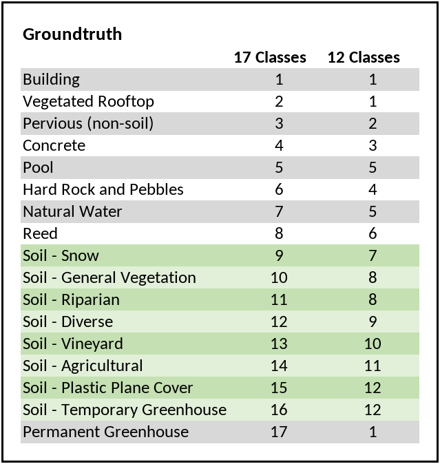
Classification Scheme

Although the goal of this project is to distinguish soil from non-soil areas, the ground truth data is classified into more detailed classes. This is due to the fact that it is easier to identify possible shortcomings of the models when the classes are more detailed. With a classification, techniques like confusion matrices can be used to identify which classes are often confused with each other, leading also to a better understanding about what areas should be covered in additional ground truth digitizations.

During development of the classification scheme, the focus lied on the distinction between soil and non-soil, which means that every class can be attributed to either soil, or non-soil, thereby respecting the legal definitions of soil according to the Federal Ordinance on Soil Pollutions⁴. The final classification scheme of the ground truth data is a product of an iterative process and has been subject of compromises between an optimal fit to the legal definitions and practical limitations like the possibility of a mere optical identification of the classes. Essentially, the scheme consists of 17 classes. However, during fine-tuning, it was found that some classes are too heavily underrepresented to be learnt by the model. As a result, the classes were merged into a new scheme consisting of 12 classes. Another feature of the classification scheme to keep in mind is that it is optimized for the Fribourgese territory, which means that some classes may not be directly applicable to other regions. The classification scheme is depicted in Figure 1.

Figure 1: Classification scheme of the ground truth data. Soil classes are depicted in green.

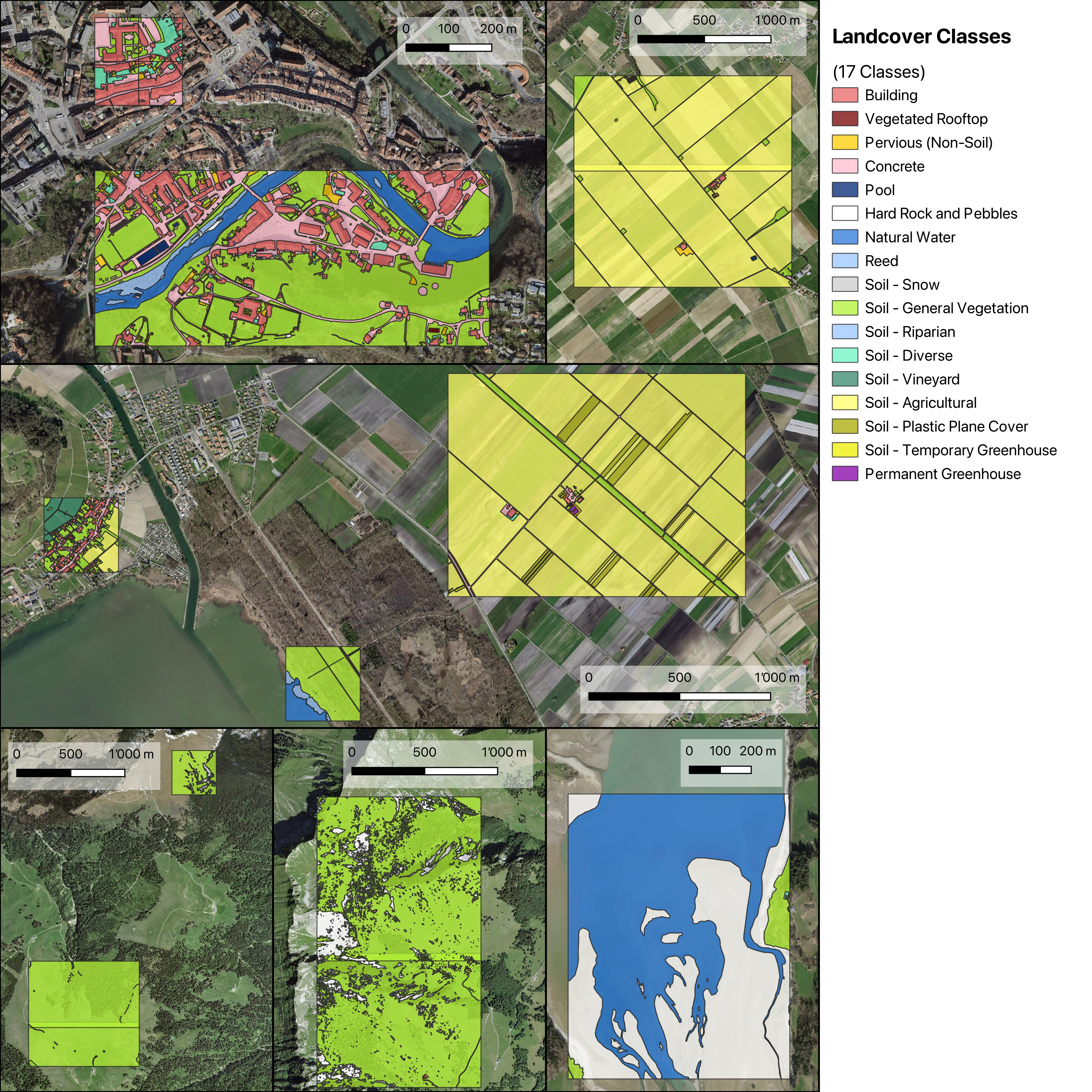
Extent

The ground truth has been digitized on the Fribourgese territory on about 9.6 km², including diverse land cover types. The area of interest is depicted in Figure 2.

Figure 2: Ground truth of the area of interest.

4. Existing Models

There are no existing models that directly fit to the project's problem: models directly outputing georeferenced, binary raster-images distinguishing soil from non-soil. However, there are models that are able to classify land cover types on aerial imagery. Three institutions have developed such models which are assessed in the evaluation section. All of them are deep learning neural networks. In the following subchapters, the models are discussed briefly.

4.1 Institut National de l’Information Géographique et Forestière (IGN)

The Département d'Appui à l'Innovation (DAI) at IGN has implemented three AI models for land cover segmentation: odeon-unet-vgg16, smp-unet-resnet34-imagenet, and smp-fpn-resnet34-imagenet, each trained with two input modalities, named RVBI and RVBIE, resulting in six configurations.

The model architectures are:

1. odeon-unet-vgg16: IGN's current production model for IGN's layer Occupation du sol à grande échelle (OCSGE). It is based on U-Net architecture with a vgg16 encoder, not pre-trained. It was trained with IGN’s own utility Odeon.
2. smp-unet-resnet34-imagenet: This U-Net architecture model uses a resnet34 encoder, pre-trained on the ImageNet dataset. It was trained with the library Segmentation Models (SMP) ⁵.
3. smp-fpn-resnet34-imagenet: Also trained using SMP, this model employs FPN architecture with a resnet34 encoder, pre-trained on ImageNet.

The input modalities are:

1. RVBI: Rouge (red) Vert (green) Bleu (blue) Infrarouge (near infrared)
2. RVBIE: Rouge (red) Vert (green) Bleu (blue) Infrarouge (near infrared) Elevation

IGN's own assessment of these 6 configurations suggests that resnet34 encoder models, with their larger receptive fields, generally outperform vgg16 models, benefiting from the spatial context in prediction. The pre-training with ImageNet further enhances model performance. Current evaluations of IGN are focusing on models from the FLAIR-1 challenge, which may replace existing models in production.

The FLAIR-1 Challenge was designed to enhance artificial intelligence (AI) methods for land cover mapping. Launched on November 21, 2022, the challenge focused on the FLAIR-1 (French Land cover from Aerospace ImageRy) dataset, one of the largest datasets for training AI models in land cover mapping. The dataset included data from over 50 departments, encompassing more than 20 billion annotated pixels, representing the diversity of the French metropolitan territory. The total area of the ground truth data is calculated as:

\[A = \frac{(512px*0.2\frac{m}{px})^2 * 77412\ tiles}{10^6} = 811.7 km^2\]

All of the used model architectures of the IGN are in the family of the convolutional neural networks (CNNs), which are a type of deep learning algorithm. Inspired by biological processes, CNNs implement patterns of connectivity between artificial neurons similar to the organization in the biological visual system. CNNs are particularly effective in image recognition tasks, as they can automatically learn features from the input data⁶.

According to IGN, the main challenges in model performance lie in adapting to varying radiometric calibrations and vegetation appearances in different datasets, such as the lack of orthophotos taken during winter (“leaf-off”) in the French training data. Ongoing efforts are aimed at improving model generalization across different types of radiometry and training with winter images to account for leafless vegetation appearances.

4.2 Haute Ecole d'Ingénierie et de Gestion du Canton de Vaud (HEIG-VD)

The Institute of Territorial Engineering (INSIT) at the HEIG-VD has participated in the FLAIR-1 challenge.

INSIT use a Mask2Former⁷ architecture, which is an attention-based model. Attention-based models in computer vision are neural networks that selectively focus on certain areas of an image during processing. They also mimic the biological visual system by concentrating on specific parts of an image while ignoring others ⁸.

The researchers at HEIG-VD could not prove a significant performance increase in including the near-infrared (NIR) channel and/or a DEM. As a result, their model works with RGB imagery only.

4.3 Office Fédéral de la Statistique (OFS)

OFS has also created a deep learning model prototype to automatically segment land cover types. However, different than the models of IGN and HEIG-VD, it works with two steps:

1. The input imagery is processed by the Segment Anything Model (SAM) by Meta ⁹. This step is used to create segments of pixels that belong to the same class without labeling the produced segments.
2. In a second step, the formerly produced segments are classified using a part of the ADELE pipeline, which is designed to automatize the acquisition of the Statistique suisse de la superficie, a point sampling grid with a mesh width of 100 meters. The data points on this grid are only representative for the exact coordinate that they lay on, not for the 100 meter square they are in, which means that the ground truth cannot be treated as an image ¹⁰. As a result, their model has been trained to classify the land cover class of only the centre pixel in an input image. To classify a segment, then, the model is used to classify a small number of sample pixels of a segment and the most frequent class is chosen as the class of the segment. The used architecture is a ConvNeXtLarge¹¹ architecture, which is a CNN. The model is limited to RGB imagery only and has been trained with a spatial resolution of 25 cm.

5. Methodology

The Methodology section describes the infrastructure used to run the models and to reproduce the project. Furthermore, it describes precisely the evaluation and fine-tuning approaches.

5.1 Infrastructure

The term “infrastrucutre” refers here to both hardware and software resources.

Hardware

Most of the development of this project was conducted on a MacBook Pro (2021) with an M1 Pro chip. To accelerate the inference and fine-tuning of the models, virtual machines (VMs) were used. The VMs were provided by Infomaniak and were equipped with 16 CPUs, 32 GB of RAM, and an NVIDIA Tesla T4 GPU.

Reproducibility

The code is versioned using Git and hosted on the Swiss Territorial Data Lab GitHub repository. To ensure reproducibility across different environments, the environment is containerized using Docker¹².

Deep Learning Framework

We received the source code and the model weights of the HEIG-VD model and of the OFS model. Both models are implemented using the deep learning framework PyTorch¹³. The HEIG-VD model uses an additional library called mmsegmentation¹⁴, which is built on top of PyTorch and provides a high-level interface for training and evaluating semantic segmentation models.

5.2 Evaluation

To realize the evaluation of the afore-mentionned models, reclassification of land cover classes into soil classes were necessary, as well as the definition of a common extent to the availabe inferences. Furthermore, the metrics were implemented in the workflow and a rigorous qualitative assessment was defined.

Inference

In the beginning of the evaluation phase, the inferences of the models were generated directly by the aforementioned institutions. Later, after receiving the model weights and the source codes, we could infere from the models of the HEIG-VD and OFS directly.

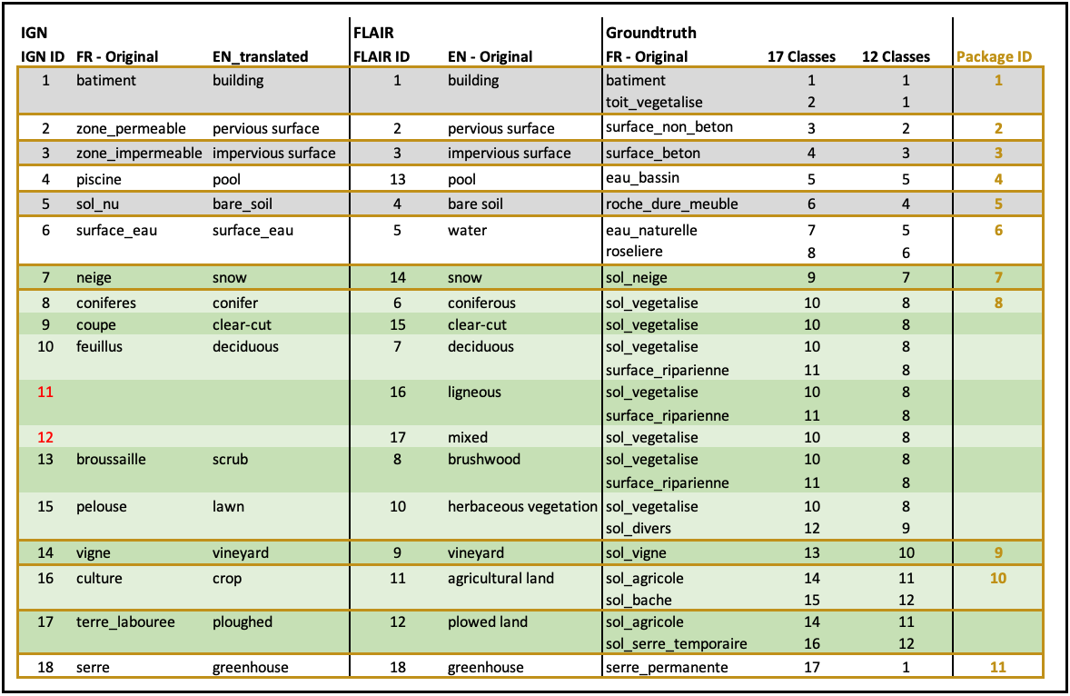
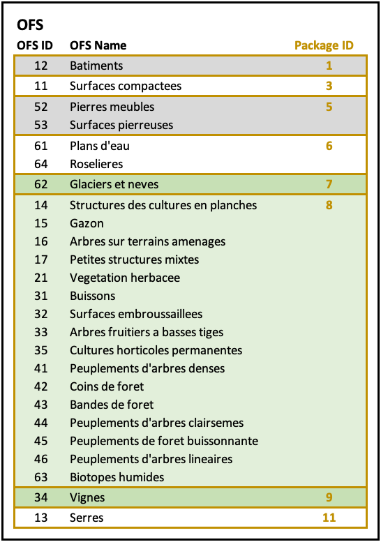
Reclassification

As already touched upon, the above-stated models do not directly output binary (soil/non-soil) raster images, but output segmented rasters with multiple classes. The classification scheme depends on the data that was used for training. The classes of the models of IGN and HEIG-VD are almost identical, since they have both been trained on French imagery and ground truth. They differ only in the numbering of the classes. The model of OFS, however outputs completely different classes. To harmonize the results of all three institution’s models and to make them fit for out problem at hand, all outputs have been reclassified to the same classification scheme named “Package ID”. The reason for this name is that there is an N:M relationship between the IGN-originated classes and the Fribourg ground truth classes. One “package” thus consists of all the classes that are connected via N:M relationships. The mapping of the classes is depicted in Figures 3 and 4.

Figure 3: Mapping between the package ID and the classification schemes of IGN and HEIG-VD.

Figure 4: Mapping between the package ID and the classification scheme of OFS.

Extents

From the extent originally covered by the ground truth, a smaller extent had to be defined during the evaluation for reasons of inferences availability and to understand the performance of the different models.

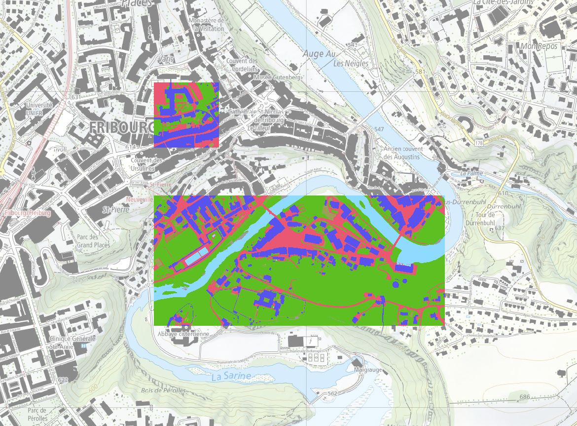
Extent 1 Because, we did not have inferences of all models for the whole area of the ground truth, we did not have the possibility to evaluate all the models on the whole extent. To allow for a fair comparison between the models, the evaluation was therefore conducted on the largest possible extent, which is the intersection between all the received inferences and the ground truth. This extent is called “Extent 1” and makes up a total area of about 0.42 km². The area can be seen in Figure 5.

Figure 5: Ground truth of Extent 1.

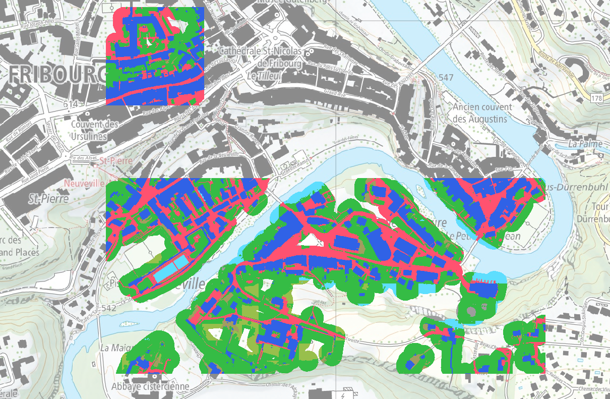
Masked Extent 1: Areas around buildings In the Extent 1, a great share of the area consists of vegetated soil. To check the performance only in the urban areas, the evaluation is also conducted for only the subset of pixels that are within 20 m of buildings. Although the extent of this modification is the same as Extent 1, it is treated like a separate extent, called “extent1-masked”, which is depicted in Figure 6.

Figure 6: Ground truth of Extent 1, masked to focus on the areas around buildings.

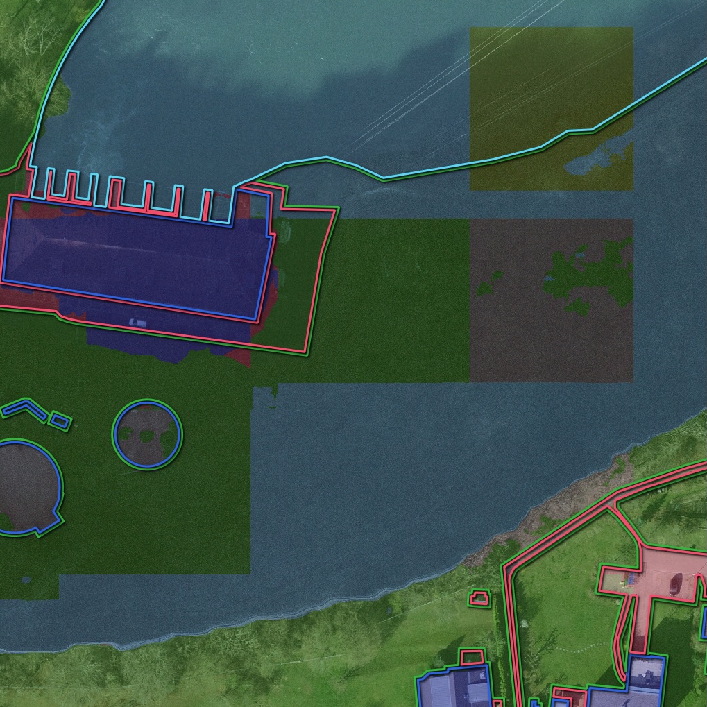
Extent 2 The output of the HEIG-VD's model is affected by square-shaped artefacts, which can be seen in Figure 7. The squares coincide with the size of the model's receptive field, which is 512x512 pixels. With an image resolution of 10 cm, the artefacts are thus of size 51.2x51.2 m, or with an image resolution of 20 cm of size 102.4x102.4 m.

There are to observations regarding the occurence of the artefacts:

1. Input tiles that are very dark and/or input tiles without much context or high-frequency texture are especially hard to classify, even for humans.
2. A sudden break between two classes in an image with only low-frequency texture is very improbable in reality. As a result, often a whole low-frequency tile is predicted to be the same class. If there is very smooth gradient of texture in the imagery on a larger scale, one whole tile could be predicted to be one class, and the next whole tile could be predicted to be another class, leading to very hard breaks in the reconnected images.

The artefacts, then, are probably a combination of those two factors.

Figure 7: Representative map showing square artefacts in areas without high-frequency context. Lines: GT, Fills: predictions

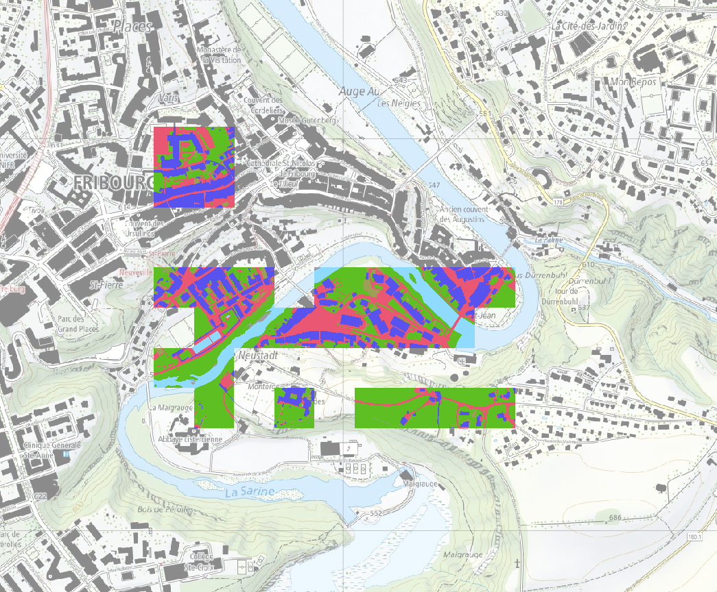
The artefacts produce large areas of false predictions that supposedly greatly influence any evaluation metric that is computed. To obtain a clearer understanding of the influence of those artefacts on the metrics, a second extent, Extent 2 as shown in Figure 8, has been created, that excludes all the tiles where the HEIG-VD model produces those artefacts.

Figure 8: Ground truth of Extent 2.

Metrics

Both the MCC and the IoU values are created in a raster-based fashion. This means that the spatially overlapping pixels of the predictions and the GT are compared to be the same. For each class, each pixel is therefore classified as one of the following:

• True Positive (TP): The pixel is correctly classified as the class.
• False Positive (FP): The pixel is incorrectly classified as the class.
• False Negative (FN): The pixel is incorrectly classified as another class.
• True Negative (TN): The pixel is correctly classified as another class.

As described in the acceptance criteria, the MCC and the IoU are then calculated as a specific combination of these values. As the MCC is only suited for a binary classification, the MCC is computed for the binary classification of the models. Only the IoU is also computed for the multiclass classification of the models. The general workflow of the evaluation pipeline is the following:

1. The models are used to predict the land cover types of the input imagery.
2. The ground truth data is rasterized to the same spatial resolution as the predictions (10cm).
3. The predictions and the ground truth data are reclassified to the same classification scheme (package ID's).
4. The predictions and the ground truth data are cut into a grid of 512x512 pixel tiles.
5. The tiles are compared, thereby computing the MCC and the IoU metrics.

More details about the technical implications of the evaluation pipeline can be found in the GitHub repository of the project.

Qualitative assessment

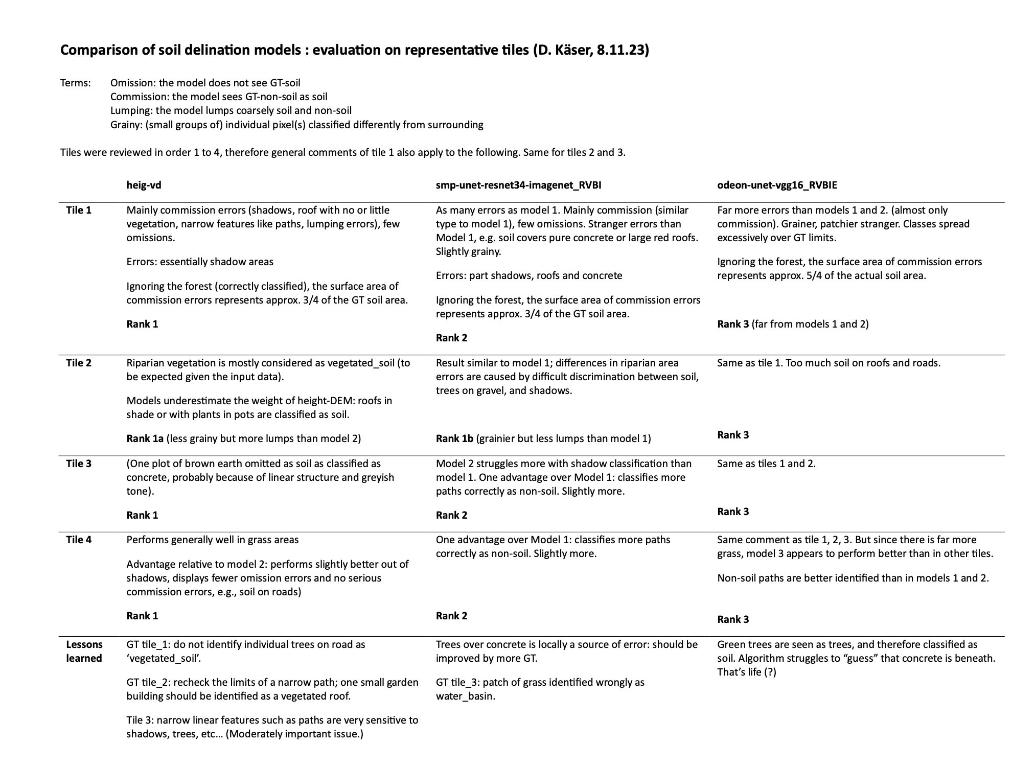
As stated in the Qualitative Assessment section, this visual assessment serves to ensure that the chosen metrics (MCC, IoU) correspond to the qualitative evaluation of the beneficiaries. Three models where chosen, such that (regarding the metrics) high- and low-performing models were included. As the problem with the artefacts in the HEIG-VD model’s predictions is very evident, for this assessment, only a subset from Extent 2 has been taken into account.

To conduct the qualitative assessment, the beneficiaries were given the predictions of the three chosen models on 4 representative tiles. The tiles were chosen to represent different land cover types (as far as possible on this area). The beneficiaries were then asked to rank the predictions of the models from best to worst.

As the inferences for the OFS model were not available at the relevant point in time, the qualitative assessment was conducted only for the IGN and the HEIG-VD models for the tiles displayed in Figure 9.

Figure 9: Tiles that were used for the qualitative assessment. Ground truth depicted as outlines, predictions as fills. IGN1: smp-unet-resnet34-imagenet_RVBI, IGN2: odeon-unet-vgg16_RVBIE.

5.3 Fine-Tuning

After the evaluation, considerations about which model to take for further progress in the project were made and the HEIG-VD model was identified as the most promising in terms of performance and availability (more in the Discussion section). The model has been trained on the FLAIR-1 dataset (see Existing Models), which differs from the present dataset in several aspects. Fine-tuning allows to retrain a model to let it adapt to the specifics of the dataset. In this case, fine-tuning aims to adjust the model to the following specifics:

• The Swiss imagery is of a higher resolution than the French imagery (10 cm vs 20 cm), which means that the model has to be able to work with more detailed information.

• The Swiss imagery is of a different season than the French imagery, which means that the model has to be able to work with different vegetation appearances.

• The classification scheme of the Swiss ground truth is different from the French ground truth, which means that the model has to be able to work with different classes.

Data Preparation

For fine-tuning, the dataset is split into the training dataset and the validation dataset. The training dataset consists of 80% of the input imagery and ground truth, while the validation dataset consists of the remaining 20%. The dataset is split in a stratified manner, which means that the distribution of the classes in the training dataset is as close as possible to the distribution of the classes in the validation dataset. This is important to ensure that the model is trained on a representative sample of the data. The split is conducted in a semi-random and tile-based manner:

1. The images are cut into a predefined grid.
2. The grid tiles are assigned to the training or validation set randomly, using different random seeds and choosing the one that leads to the most even class frequency distribution.
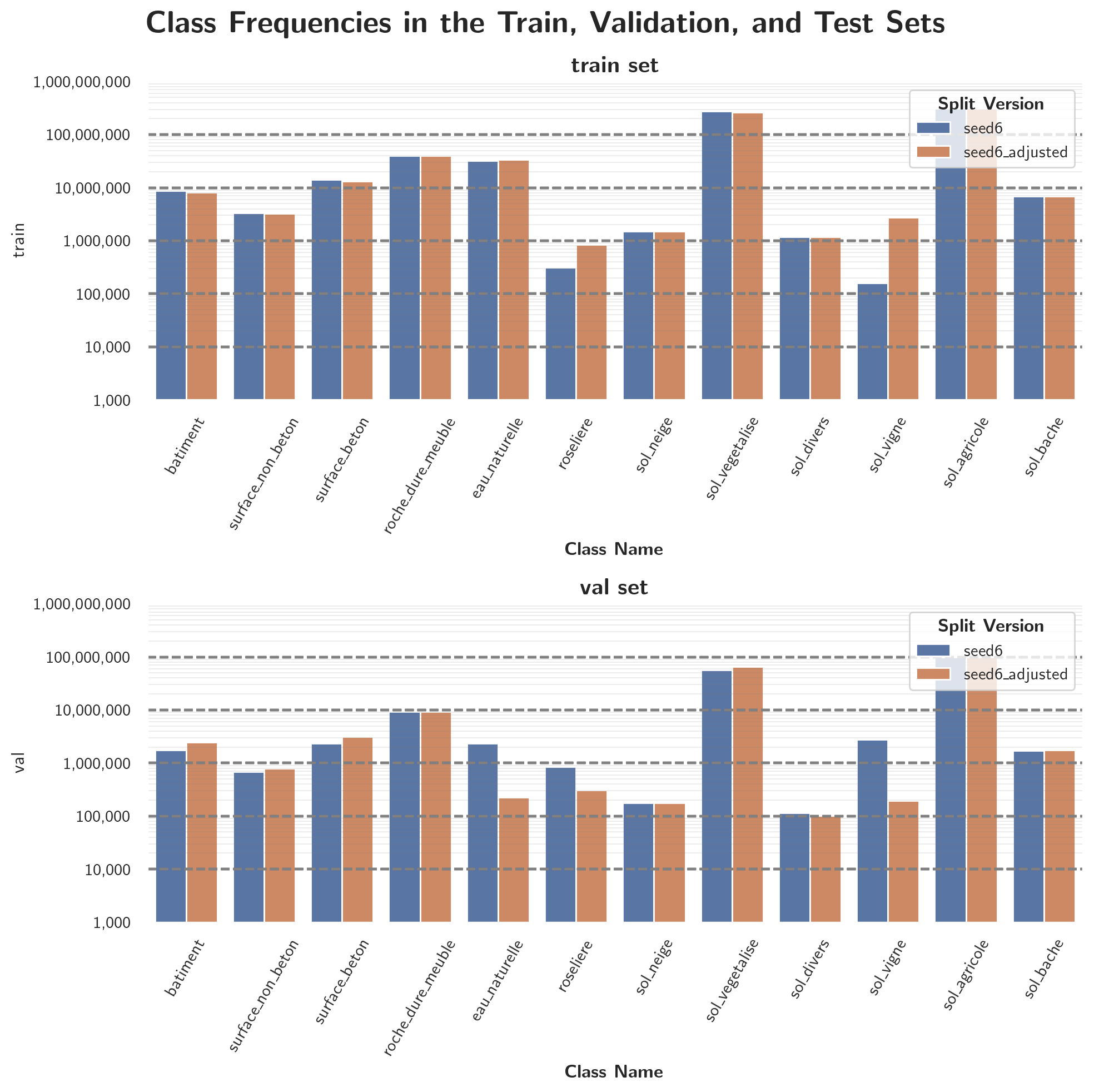
3. After identifying the seed 6 as the best one, the split was manually adjusted to ensure that the class frequency distributions of the two datasets are as representative as possible. The final distribution can be seen in Figure 10. Only the class frequencies of the class sol_vigne and roseliere change considerably.

As stated in the Ground Truth section, the fine-tuning is conducted using the classification scheme consisting of 12 classes.

Figure 10: Class frequency distribution of the training and validation dataset. Mind that the y-axis is logarithmic.

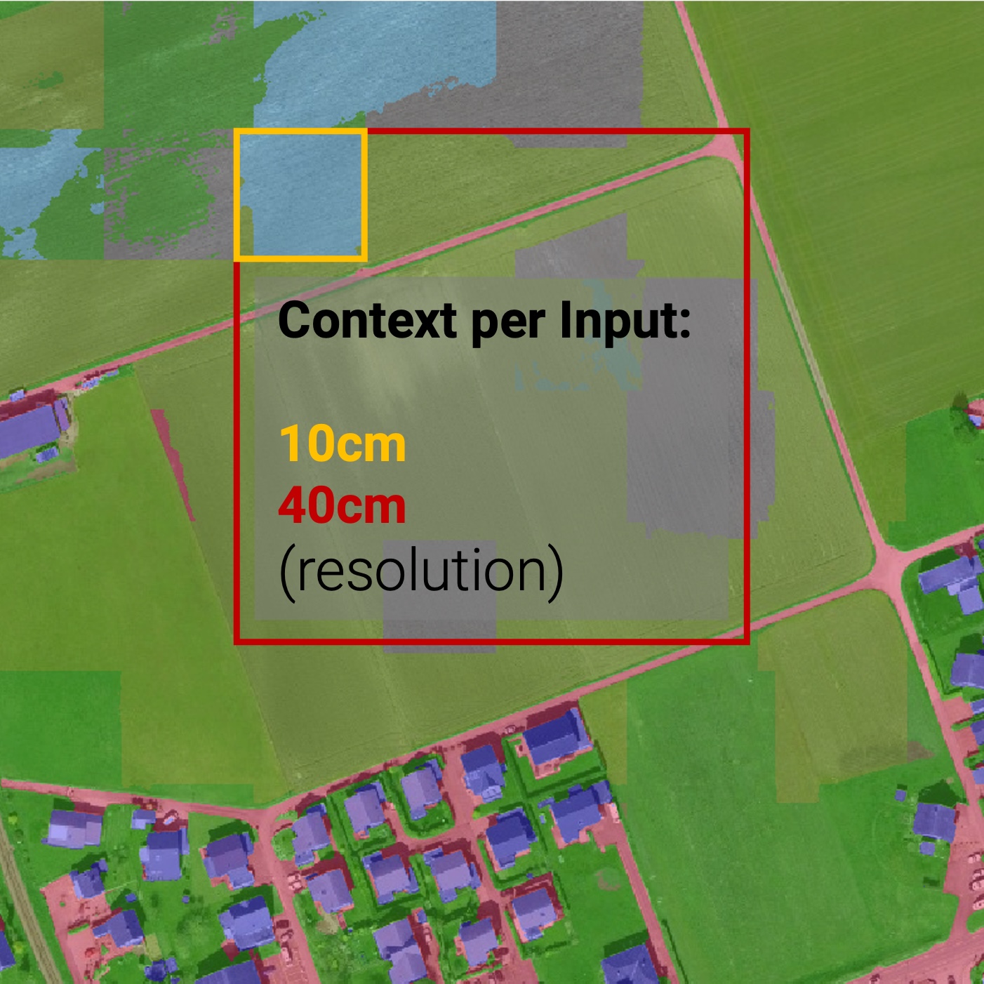
To mitigate the effect of the artefacts, mentioned in the Extent section, we propose to decrease the spatial resolution of the input (and thus also the output) of the model to increase the spatial receptive field of the model. With input tiles covering a larger area, the chance of the occurrence of high-frequency features that give context to the image increases. A visualization of this proposal is shown in Figure 11: while the 10 cm input tile has only low-frequency agricultural context, the 40 cm input tile has high-frequency context in the form of a road. This context, as proposed, could help the model to make a more informed decision.

Figure 11: Visualization of the changing receptive field of the model with different input resolutions

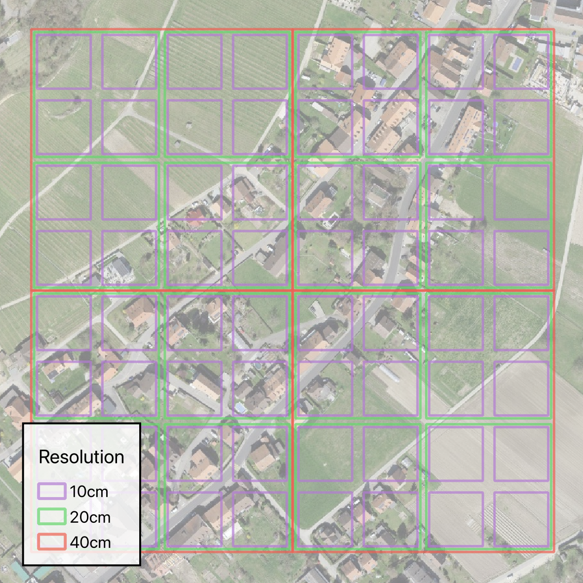
As a model adjusts for a certain resolution during training, we test the effect of training on different resolutions. Thus, the model is fine-tuned on two different datasets, one with a spatial resolution of 10 cm and one with mixed resolutions of 10 cm, 20 cm, and 40 cm. The input shape of all the image tiles, regardless of the ground sampling distance, is 512x512 pixels. The spatially largest tiles (40 cm) were assigned to either the training or the validation set, and all the smaller tiles that are contained within the larger tiles were assigned to the same set. This way, the model can be trained and evaluated, respectively, on the same area at different resolutions. The resulting nested grid is depicted in Figure 12.

Figure 12: Example of the used grid. The shape of the tiles is always 512 by 512 pixels, only the ground sampling distance changes. Borders have an offset to increase legibility, in reality, they're perfectly overlapping.

The obtained datasets and their sizes are summarized here:

• Training Dataset

  • 10cm: 2'640 tiles
  • 20cm: 656 tiles
  • 40cm: 164 tiles
  • Mixed: 3'460 tiles

• Validation Dataset

  • 10cm: 692 tiles
  • 20cm: 172 tiles
  • 40cm: 43 tiles
  • Mixed: 907 tiles

Training

Both the models trained on the single-resolution and on the mixed-resolution dataset have been trained for a total of 160'000 iterations using the mmsegmentation library¹⁴. One iteration in this context means one batch of data has been processed. Because of memory limitations, the models were trained with a batch-size of 1, which means, that one iteration corresponds to one tile being processed. Thus, one epoch (one pass through the whole dataset) consists of 2'640 iterations for the single-resolution dataset and 3'460 iterations for the mixed-resolution dataset. During training, the models were evaluated on the validation set after every epoch by computing the mIoU metric. If the mIoU increased, a model checkpoint was saved and the old one deleted. After training for the predefined number of iterations, the model with the highest mIoU on the validation set was chosen as the final model.

6. Results

The metrics values for the evaluation and the fine-tuning parts of the project are first presented. Afterwards, a close view of the final product is shown.

6.1 Evaluation

The multiclass evaluation is briefly presented before showing in details, from a quantitative and qualitative perpectives, the evaluation of the models for the binary classification in soil and non-soil classes.

Multiclass Evaluation

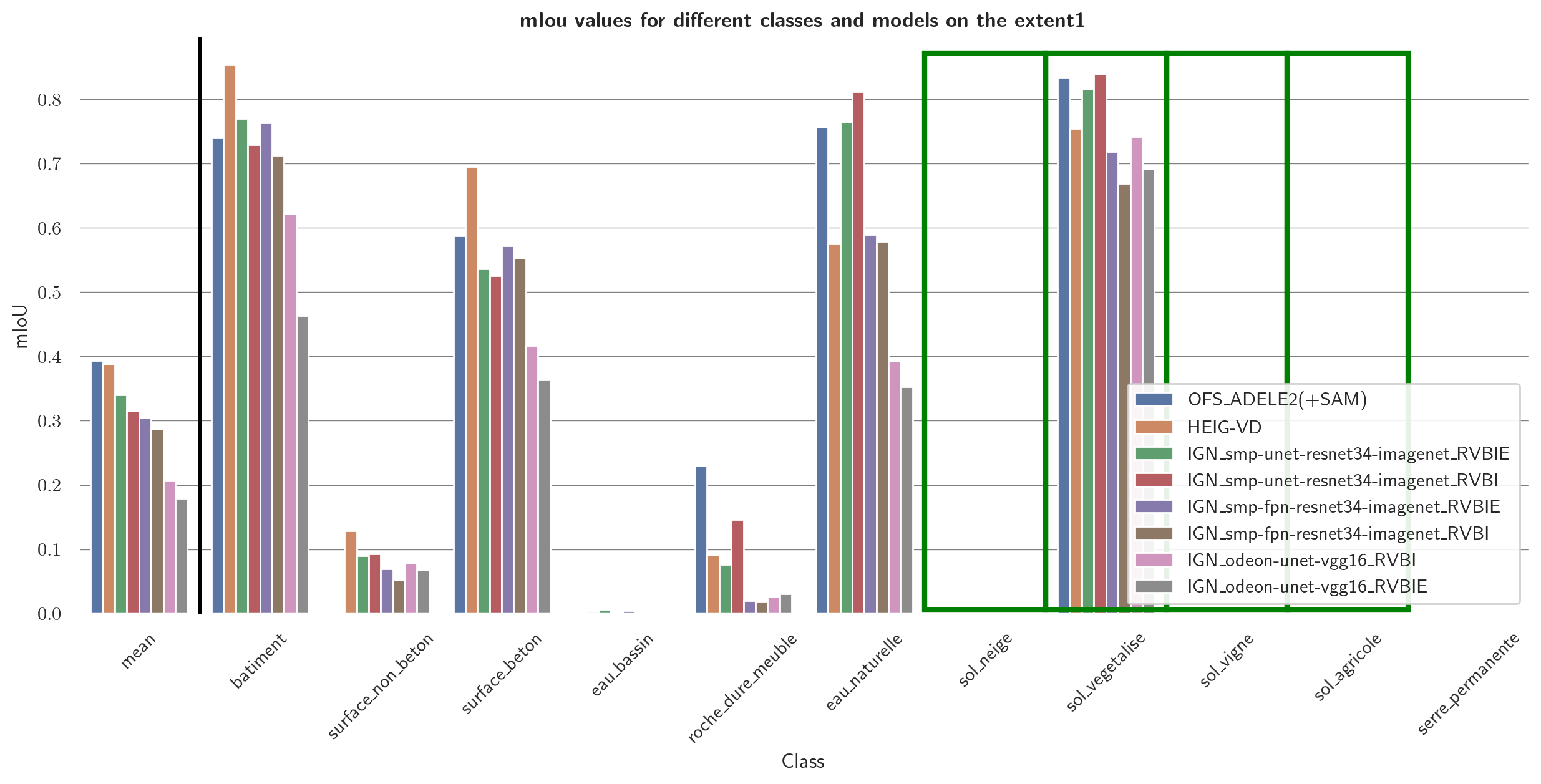
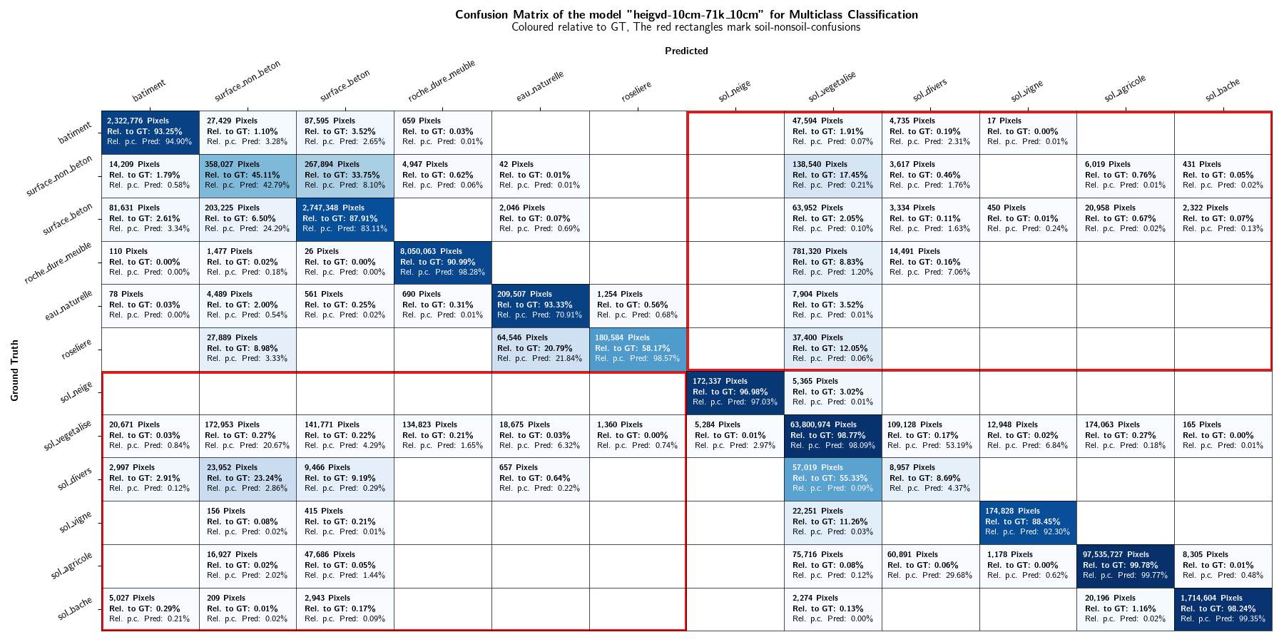
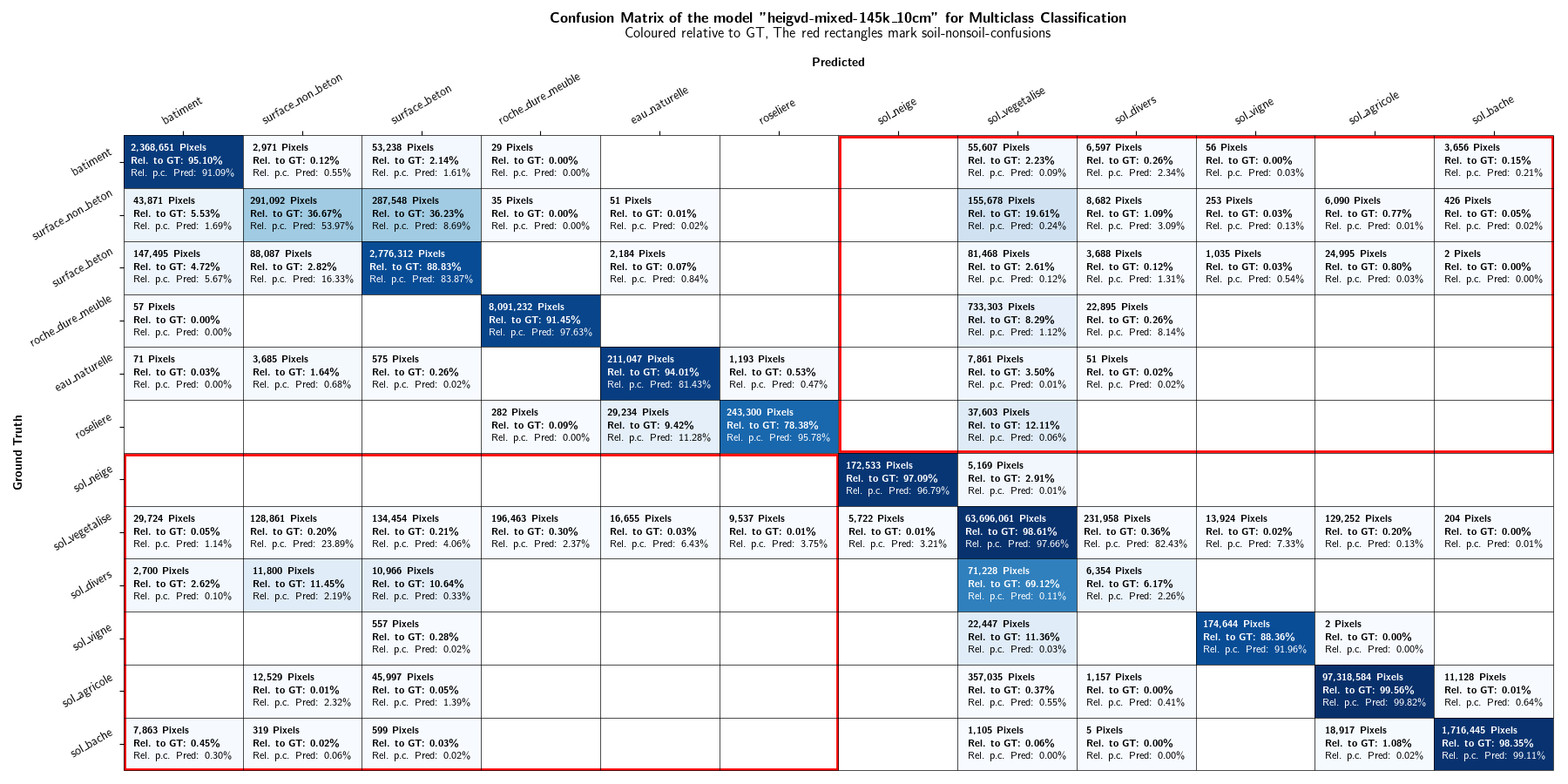
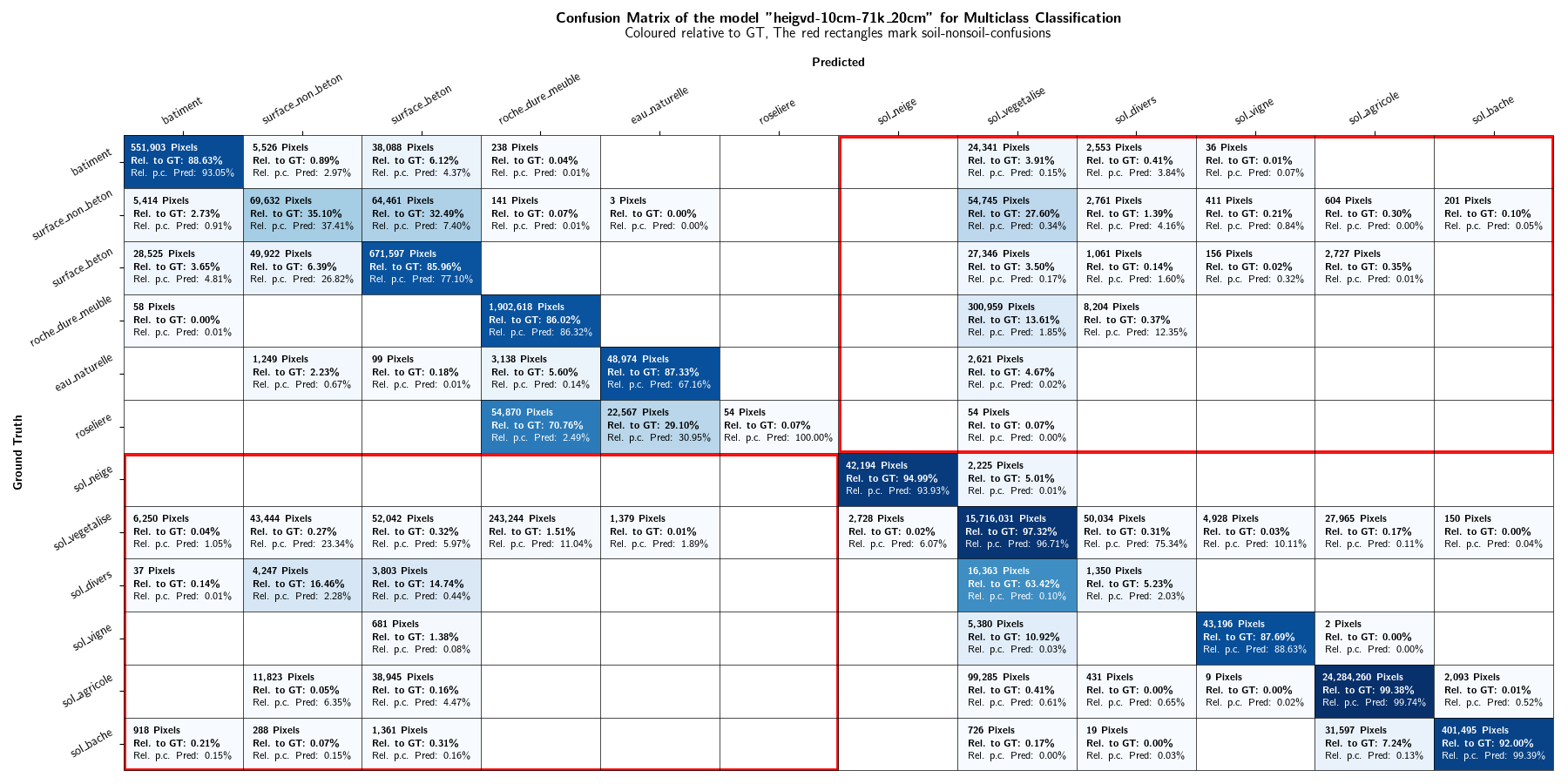
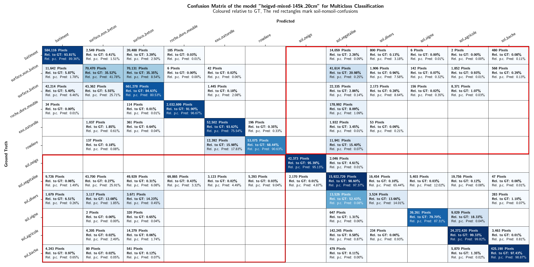
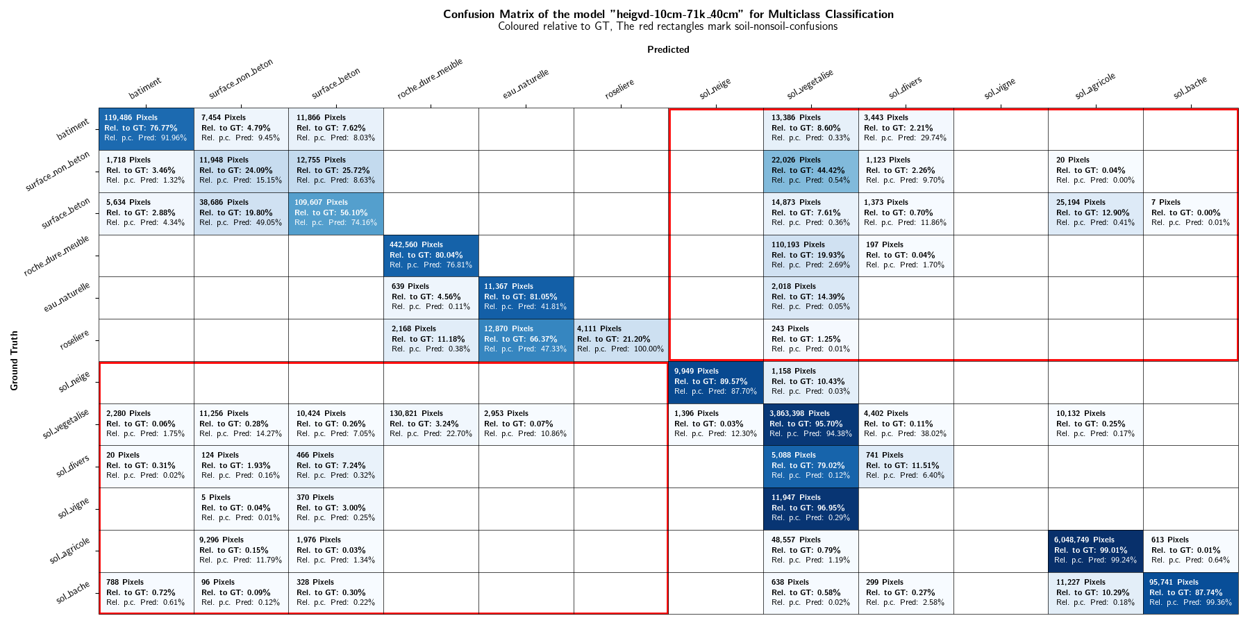
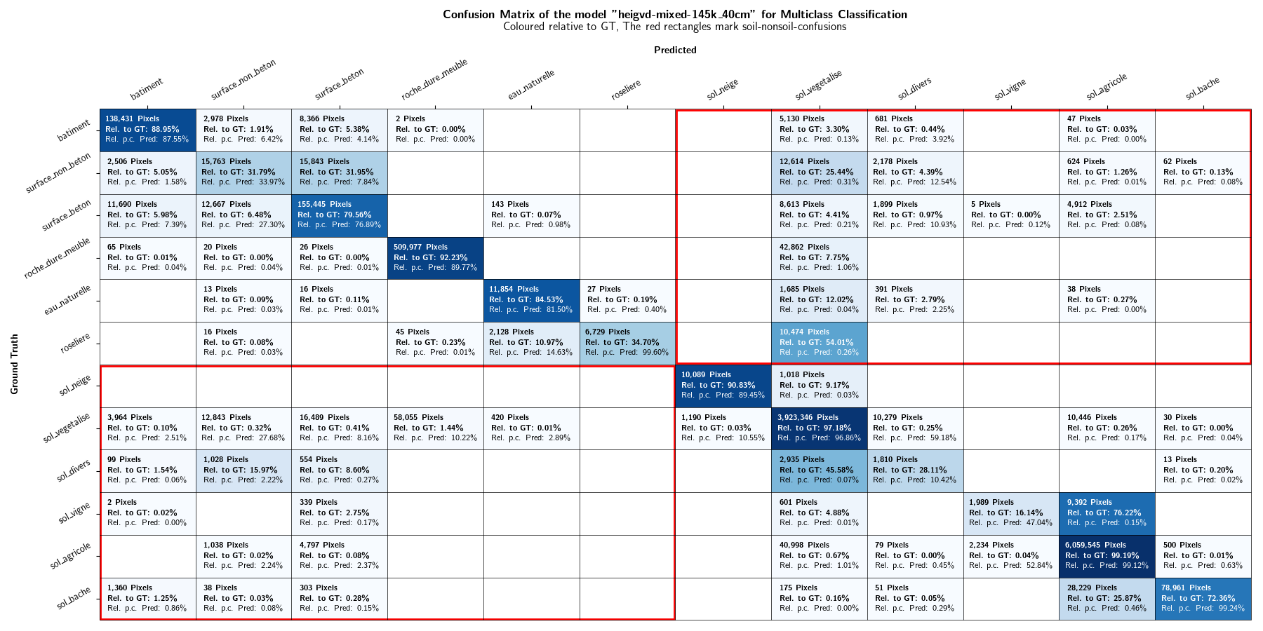
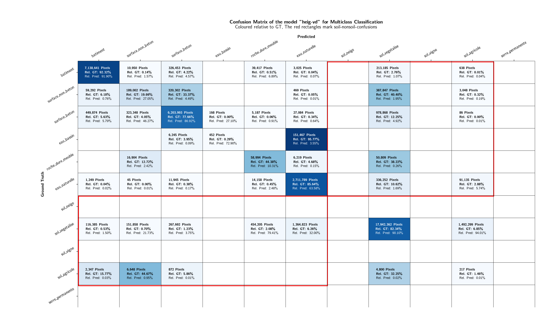
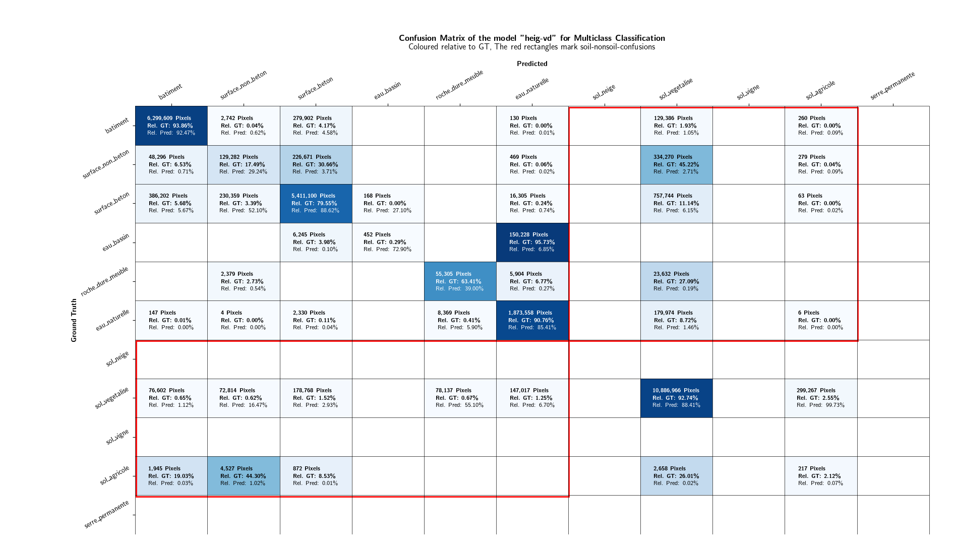
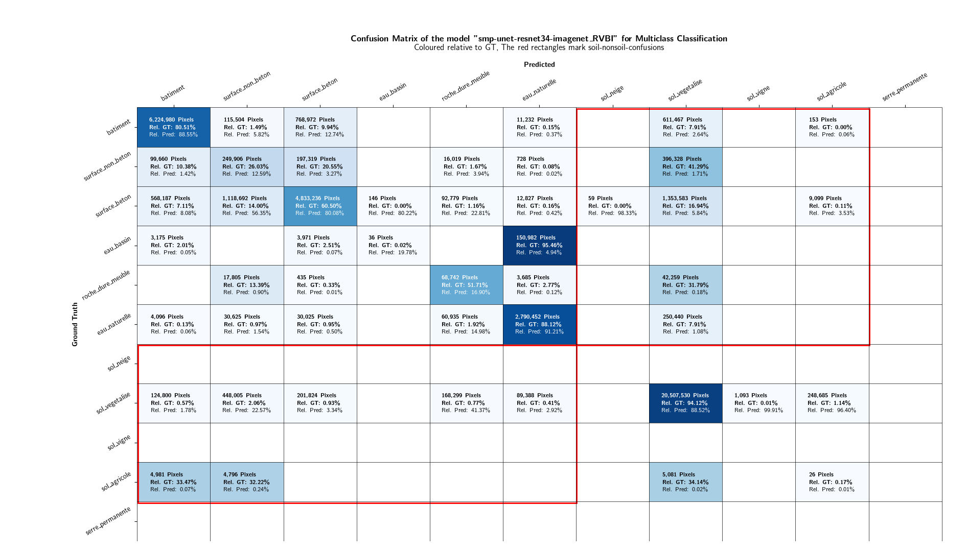
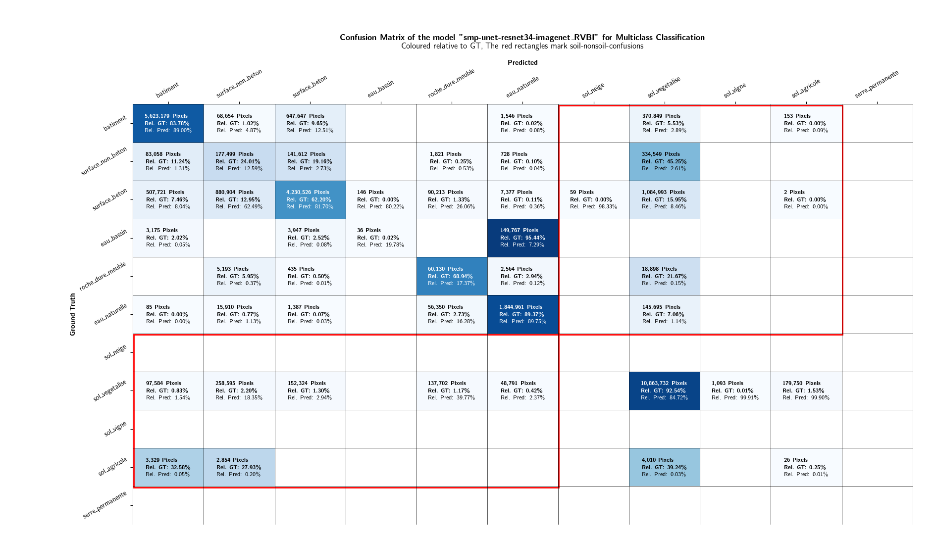
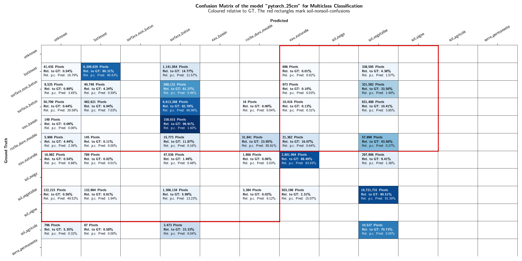
As the focus of this project lies in the binary distinction between soil and non-soil areas, the multiclass classification results are not discussed in further detail. However, plots displaying the class-IoU values of the different models are depicted in Figures 13 and 14. Confusion matrices can be found in the Appendices.

Figure 13: IoU values for different models and classes on Extent 1. Soil-classes are depicted in the green rectangles.

Figure 14: IoU values for different models and classes on Extent 2. Soil-classes are depicted in the green rectangles.

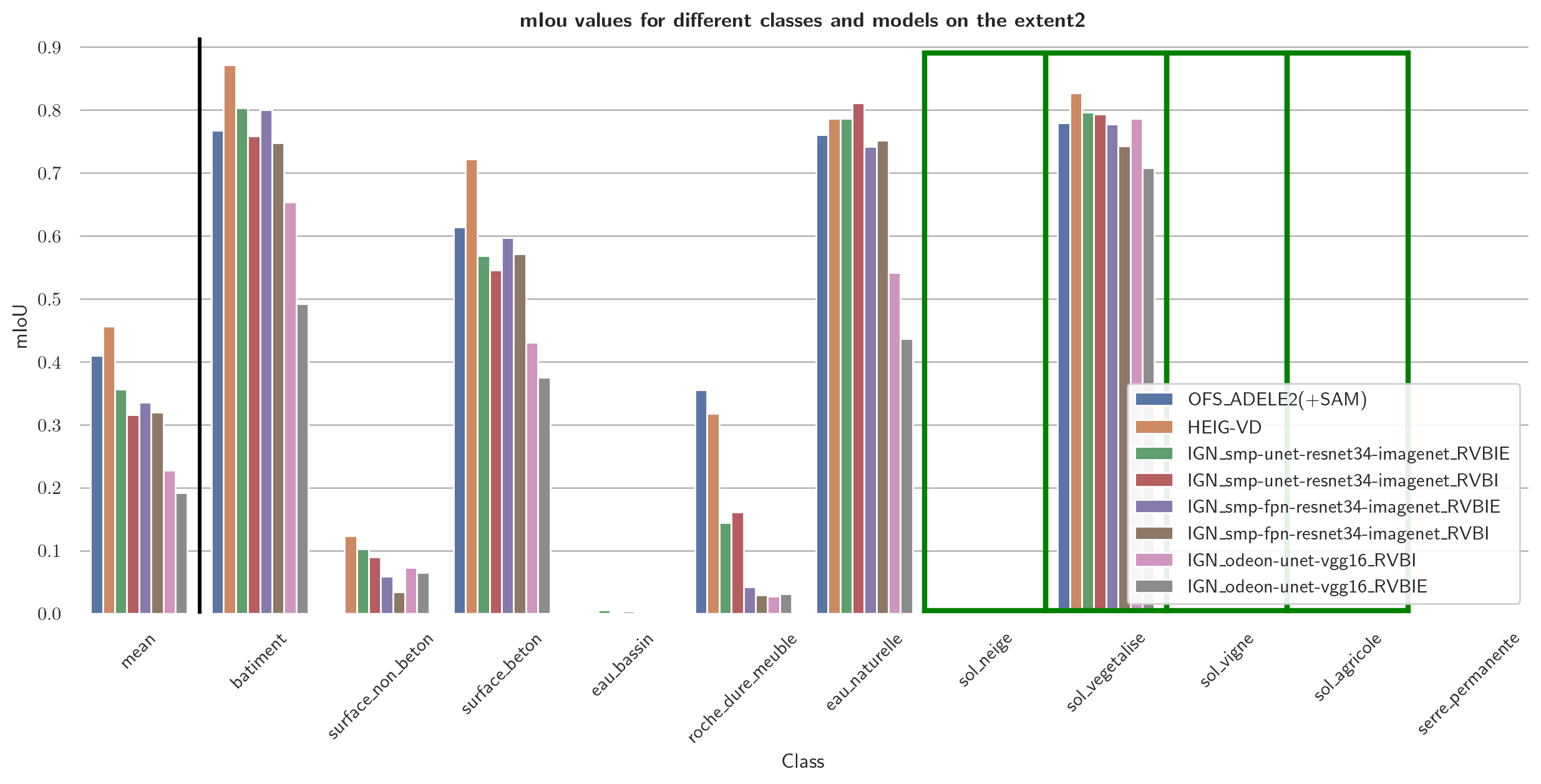
Quantitative Evaluation

Figure 15 and 16 show the MCC values and mIoU values, respectively, computed for the binary classification of different models. As the distribution of the metrics across the models is very similar, only the MCC values are discussed in the following and are precisely given in Table 1.

Figure 15: MCC values of the binary predictions of the models on the two extents.

Figure 16: mIoU values of the binary predictions of the models on the two extents.

Model	MCC (Extent 1)	MCC (Masked Extent 1)	MCC (Extent 2)
IGN_smp-unet-resnet34-imagenet_RVBI	0.825	0.808	0.813
OFS_ADELE2(+SAM)	0.818	0.802	0.794
IGN_smp-unet-resnet34-imagenet_RVBIE	0.810	0.798	0.824
HEIG-VD	0.789	0.839	0.859
IGN_smp-fpn-resnet34-imagenet_RVBIE	0.714	0.749	0.795
IGN_odeon-unet-vgg16_RVBI	0.710	0.706	0.794
IGN_smp-fpn-resnet34-imagenet_RVBI	0.710	0.745	0.792
IGN_odeon-unet-vgg16_RVBIE	0.640	0.613	0.713

Table 1: MCC of the binary predictions of the models on the three extents.

Extent 1 The best-performing model in Extent 1 is the IGN_smp-unet-resnet34-imagenet_RVBI model, with an MCC of 0.825. The inclusion of the elevation channel does not seem to have a significant impact on the model's performance, as the IGN_smp-unet-resnet34-imagenet_RVBIE model only achieves an MCC of 0.810. The OFS_ADELE2(+SAM) model follows closely with an MCC of 0.818. The HEIG-VD model, on the other hand, performs significantly worse, with an MCC of 0.789. The models IGN_smp-fpn-resnet34-imagenet_RVBIE, IGN_odeon-unet-vgg16_RVBI, and IGN_smp-fpn-resnet34-imagenet_RVBI all achieve an MCC of around 0.710. The IGN_odeon-unet-vgg16_RVBIE model performs the worst, with an MCC of 0.640.

masked Extent 1 & Extent 2 The greatest difference to Extent 1 is that in masked Extent 1 and in Extent 2, the HEIG-VD model performs significantly better than in masked Extent 1, with an MCC of 0.839. Generally, the models perform similarly in masked Extent 1 and in Extent 1. The models are generally performing better in Extent 2.

Qualitative Evaluation

The results of the qualitative assessment are depicted in Figure 17. The qualitative assessment rendered the following ranking:

1. heig-vd
2. smp-unet-resnet34-imagenet_RVBI
3. odeon_unet-vgg16_RVBIE

The ranking corresponds to the ranking based on the metric measures.

Figure 17: Qualitative assessment by the beneficiaries.

6.2 Fine-Tuning

For the second part of the project - fine-tuning of the HEIG-VD model - the quantitative binary performance is first presented. Afterwards, the multiclass outputs are quantitatively, qualitatively and visually given. This allows to understand what is behind the visual binary outputs qualitatively discussed it the final subsection.

Binary Results

Figure 18 shows the progress of the models during fine-tuning, with a datapoint after every epoch. The curves are quite similar to each other, but both are rather noisy. The best checkpoint of the 10 cm model is at epoch 71 with an mIoU of 0.939. The best checkpoint of the mixed model is at epoch 145 with an mIoU of 0.930. The names of the two models are thus HEIG-VD-10cm-71k and HEIG-VD-mixed-145k.

The training for the models for 160'000 iterations with the above stated hardware took about 7 days. Performing inference on one single tile with 512x512 pixels takes about 1 second. This means that with 10 cm input tiles, the model takes about 380 seconds or 6 minutes and 20 seconds to process 1 km². As the canton of Fribourg has an area of about 1'670 km², the model would take about one week to process the whole canton. The model would able to process the whole canton in a reasonable amount of time.

Figure 18: Training progress of the models.

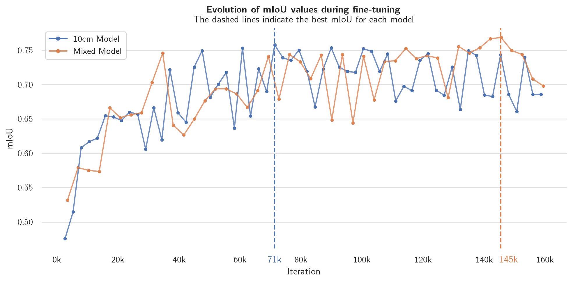
Figure 19 and Table 2 show the MCC values for the original HEIG-VD model, as well as for the two fine-tuned models one the evaluation extent. When comparing the MCC values of the original HEIG-VD model (MCC=0.553) with the fine-tuned models (MCC after 10 cm training : 0.939; MCC after mixed training: 0.938 ), the fine-tuned models perform significantly better. However, one should notice that the original HEIG-VD model was trained on a different dataset and with a different classification scheme. It was evaluated on the same extent but using the package ID, which is introduced in the Reclassification section.

Regarding the performance of the two models on inference with different input resolutions, they perform quite similarly on the 10 cm resolution input. Both models perform worse as the ground sampling distance increases:

• MCC after 10 cm training: 0.884 on 20 cm inputs against 0.795 on 40 cm inputs.
• MCC after mixed training: 0.930 on 20 cm inputs against 0.893 on 40 cm inputs.

However, the performance of the HEIG-VD-mixed-145k model is not decreasing as much as the HEIG-VD-10cm-71k model on the 20 cm and 40 cm resolution inputs.

Figure 19: MCC values of the binary predictions of the model fine-tuned on different resolutions.

Model	MCC (10cm input)	MCC (20cm input)	MCC (40cm input)
HEIG-VD-original	0.553
HEIG-VD-10cm-71k	0.939	0.884	0.795
HEIG-VD-mixed-145k	0.938	0.930	0.893

Table 2: MCC values of the binary predictions of the model fine-tuned on different resolutions.

Multi-Class Results

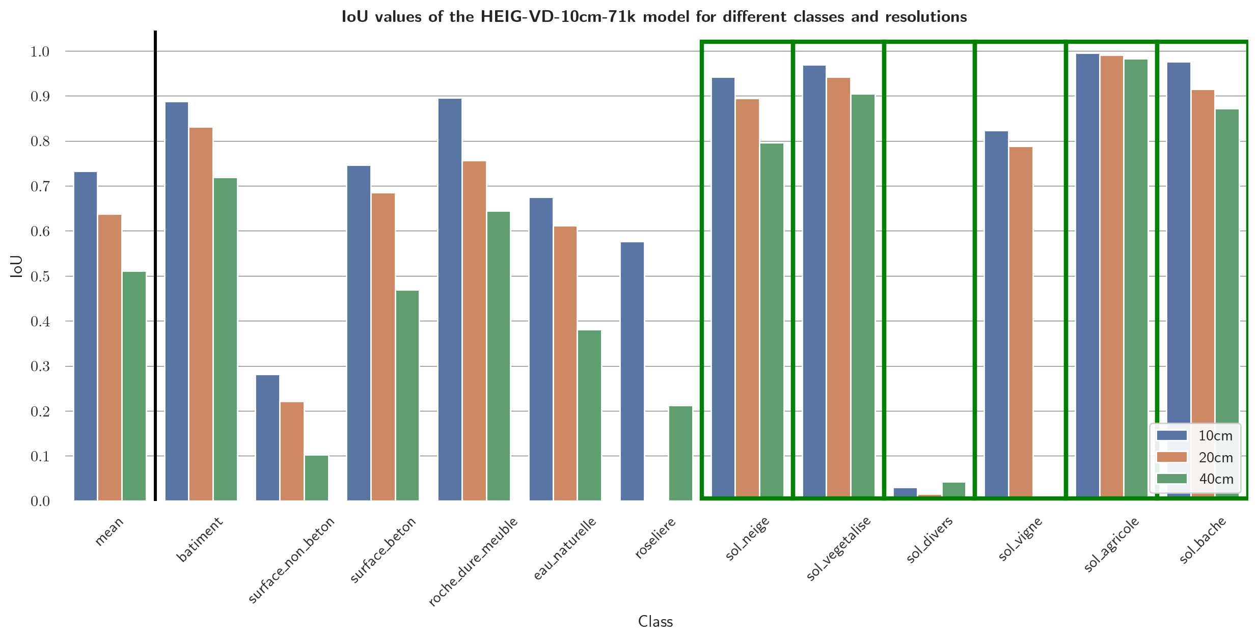
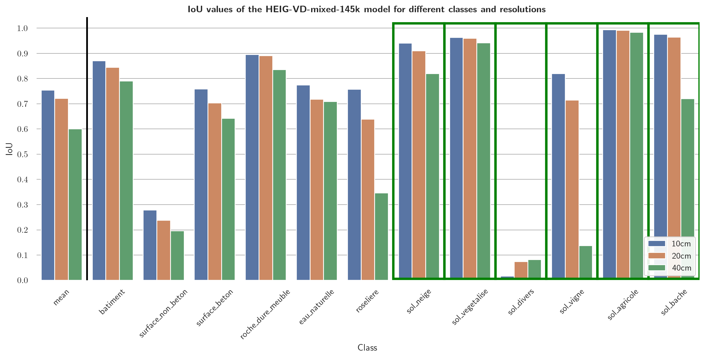
As in the Evaluation results section, the results are not discussed in further details. Confusion matrices can be found in the Appendices. Figures 20 and 21 shows the IoU values of the mixed-resolution model (Figure 20) and the 10 cm model (Figure 21) on different resolutions.

Figure 20: IoU values of the fine-tuned models on the 10 cm dataset.

Figure 21: IoU values of the fine-tuned models on the mixed-resolution dataset.

Qualitative Analysis of the Outputs

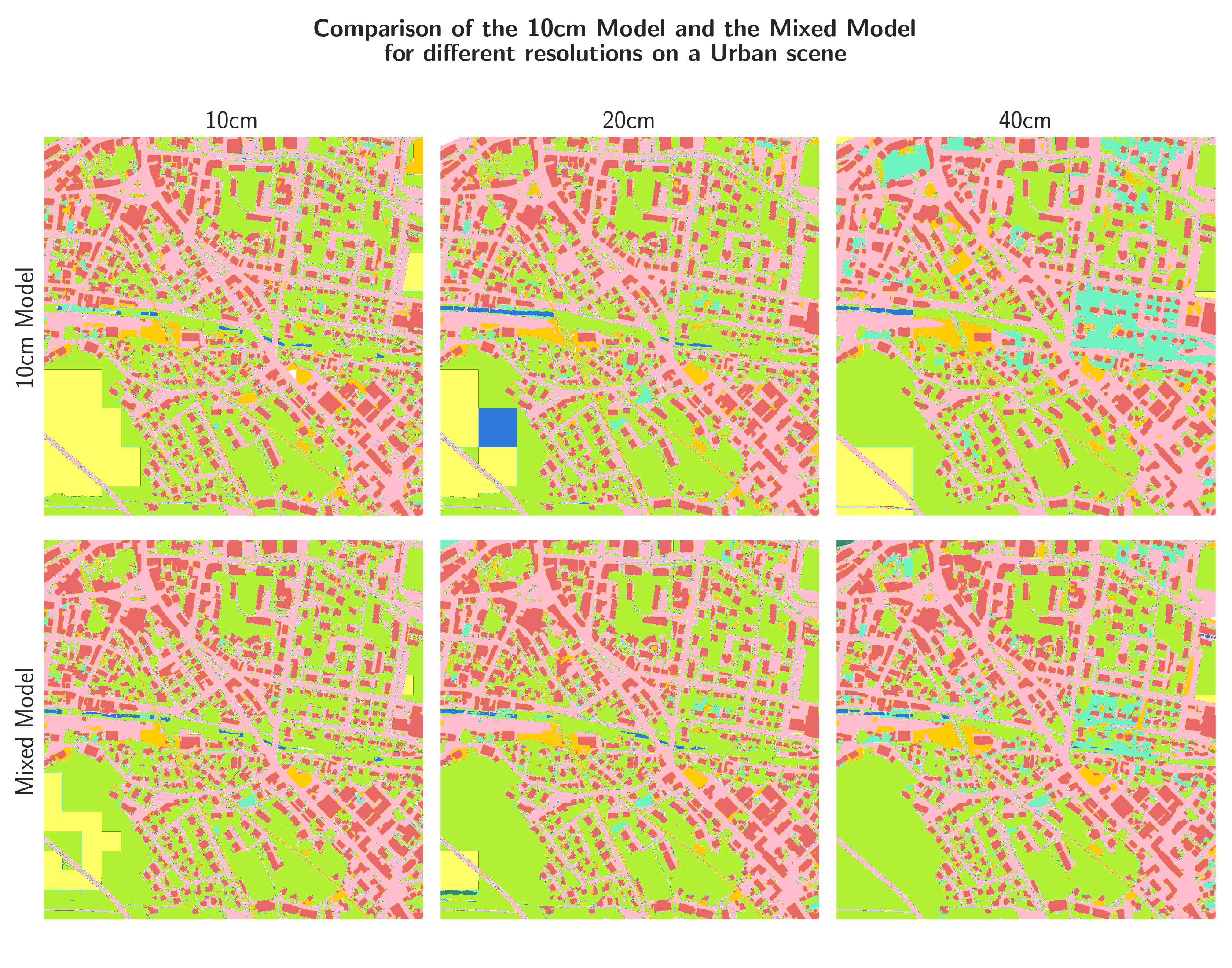
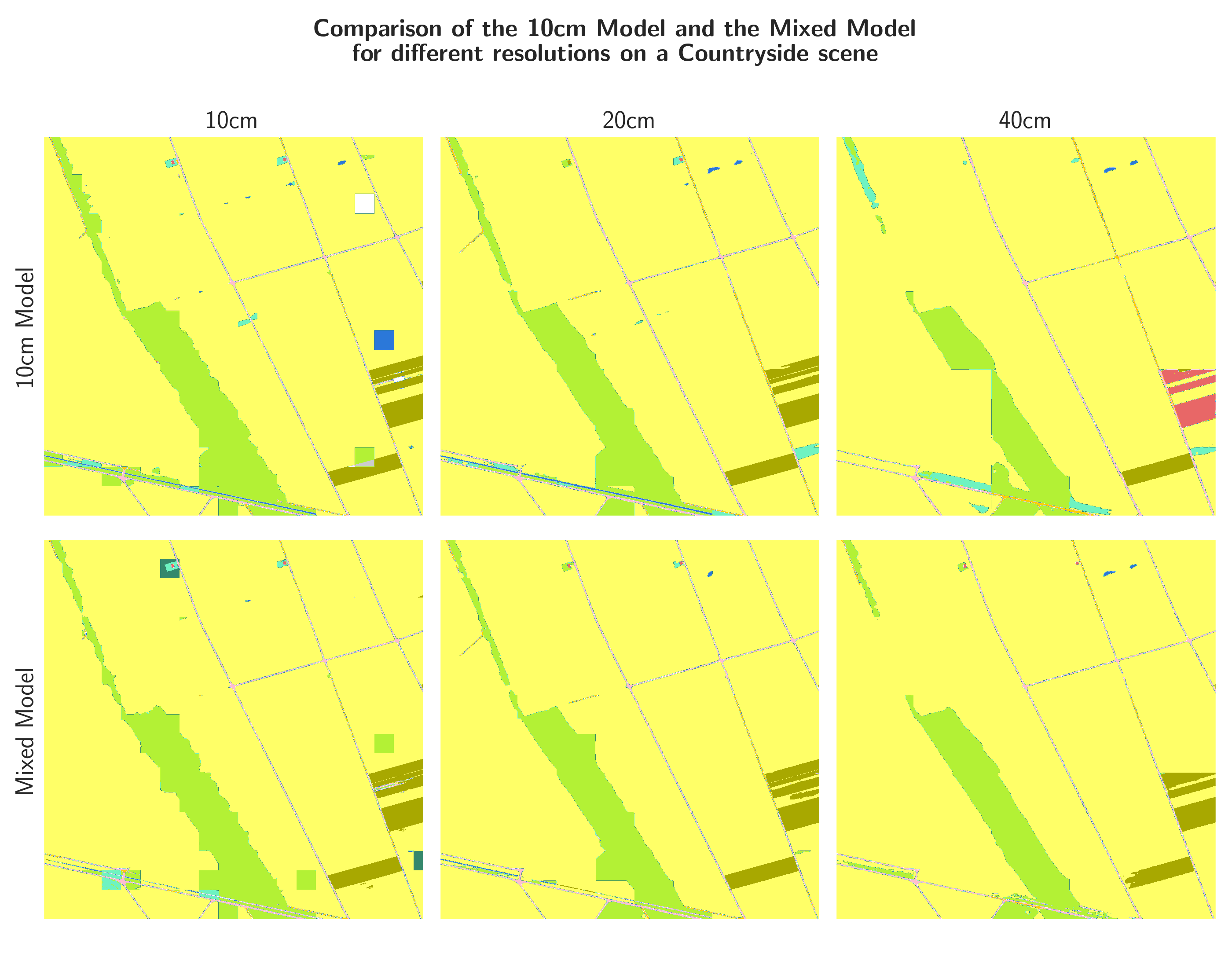
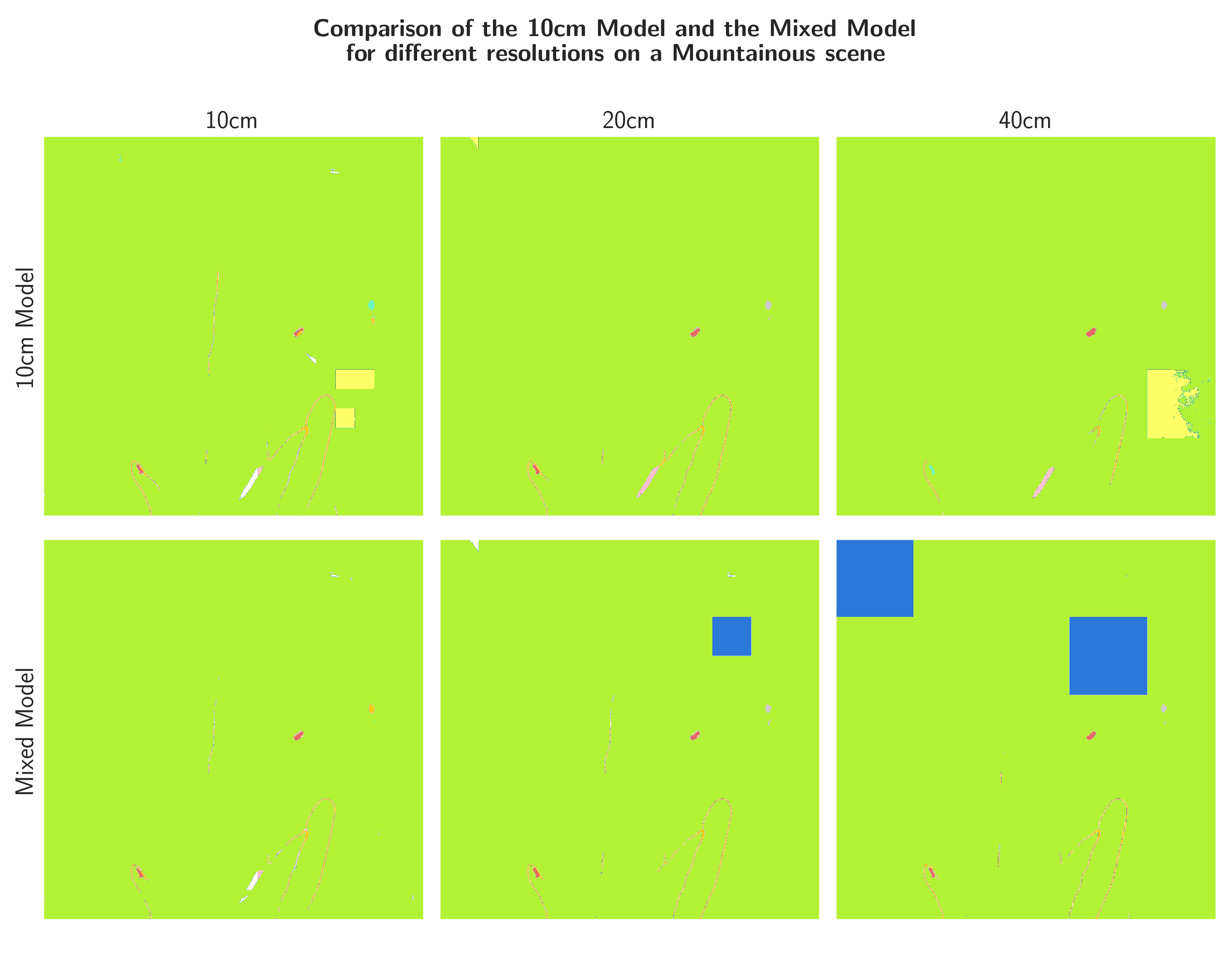
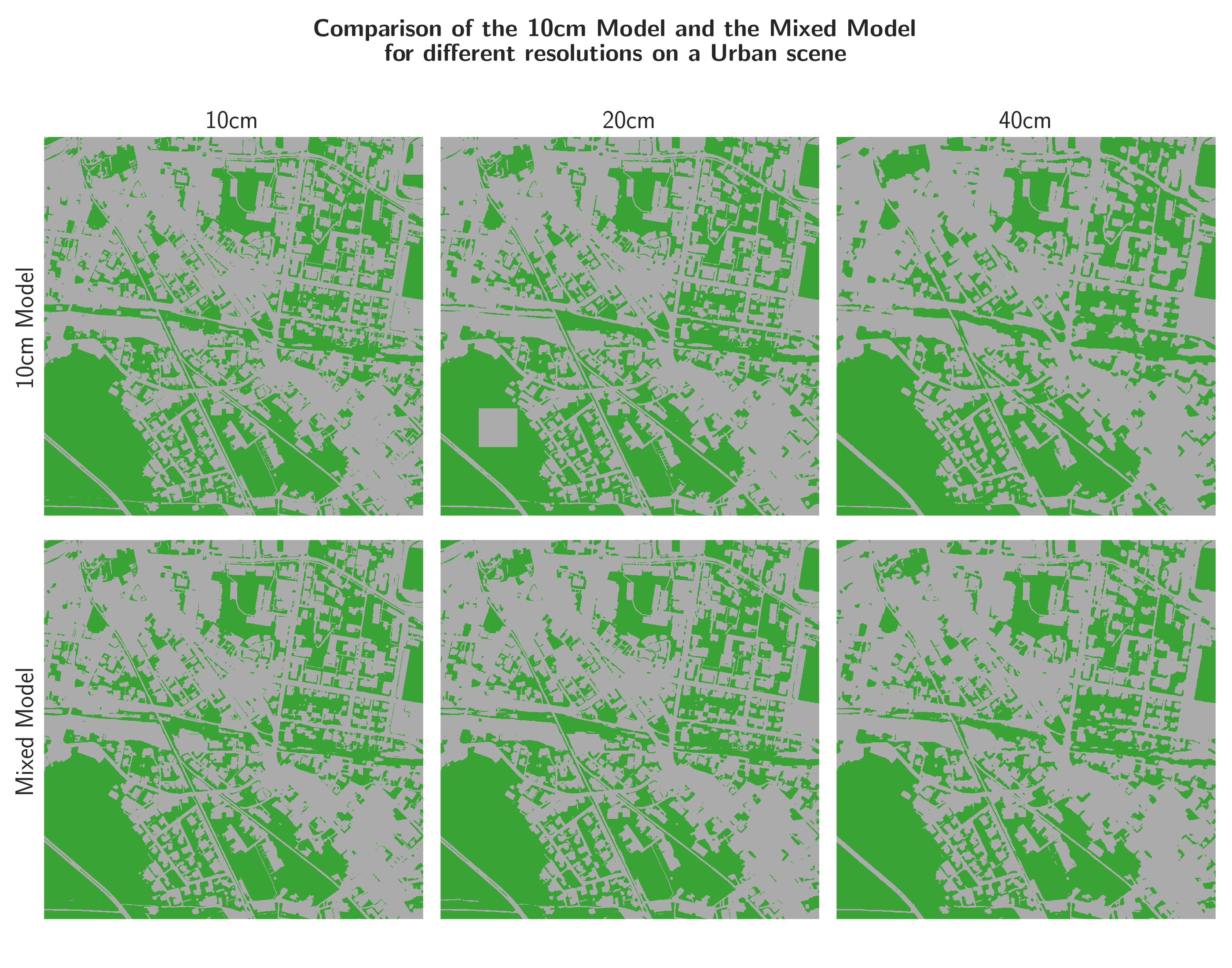
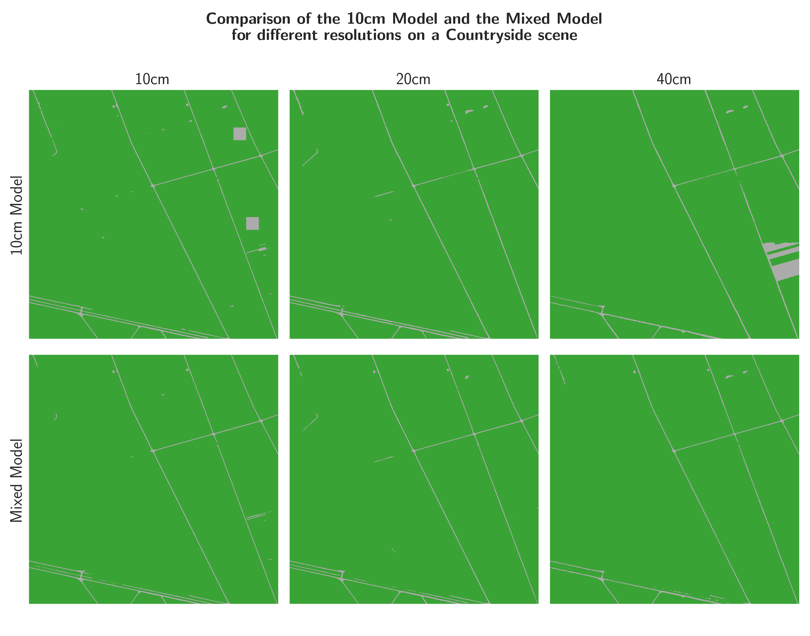
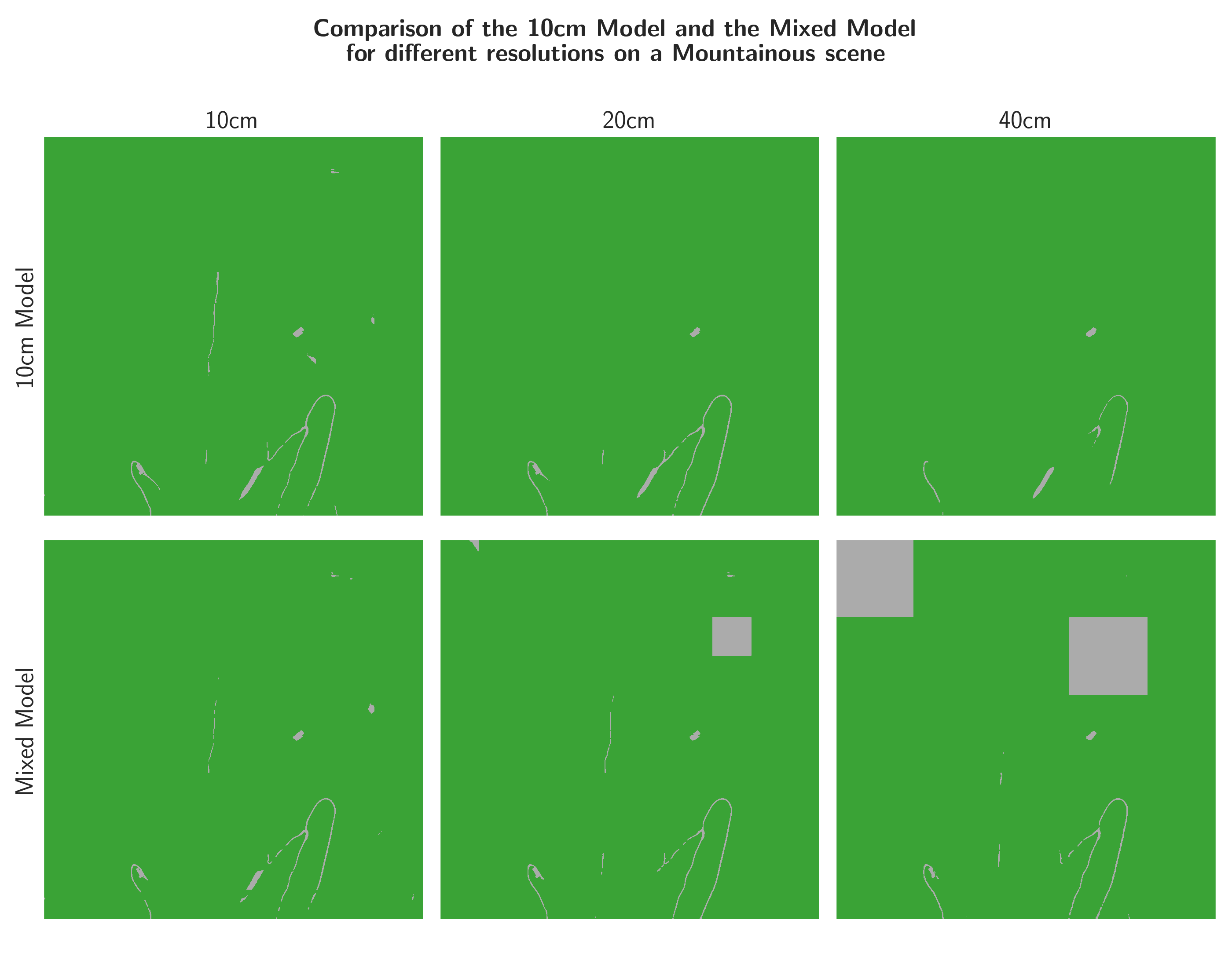
Figures 22, 23, and 24 show the outputs of the two models for 10, 20, and 40 cm input resolution, respectively, on three different areas. The areas were chosen to represent different land cover types. Since there is no ground truth on this areas, these inferences can only be analyzed qualitatively. On the inferences it is apparent, that the models still have trouble on regions with little high-frequency context and are prone to square artefacts. In the urban and countryside areas (Figure 22 and 23), the combination of decreased resolution (and thus increased spatial receptive field) and the fine-tuning on the mixed dataset seems to have a positive effect on the occurrence of the square artefacts. In the mountainous area (Figure 24), however, the artefacts are even more pronounced in the outputs of the mixed-resolution model than in the 10cm-only model.

An effect of the decreased resolution is that, generally, the predictions seem to be less impacted by the artefacts. However, if there are artefacts, their spatial extent, being the same as the spatial receptive field of the model, is larger.

Figure 22: Comparison of the predictions of the model fine-tuned on different resolutions in urban areas.

Figure 23: Comparison of the predictions of the model fine-tuned on different resolutions in countryside areas.

Figure 24: Comparison of the predictions of the model fine-tuned on different resolutions in mountainous areas.

Qualitative Analysis of the Binary Outputs

Figures 25, 26, and 27 show the binary output versions of the three Figures above (22, 23, and 24). Looking at the inferences on the same areas, one can see that the artefacts are much less of an issue in the binary outputs. They are still present to some extent, however, since many of the artefacts and their surroundings are in fact soil, or non-soil, respectively, the artefacts dissolve in the binary outputs. The artefacts are still present in the mountainous area where the mixed model predicts large areas of water, which is a non-soil class.

Figure 25: Comparison of the binary predictions of the model fine-tuned on different resolutions in urban areas.

Figure 26: Comparison of the binary predictions of the model fine-tuned on different resolutions in countryside areas.

Figure 27: Comparison of the binary predictions of the model fine-tuned on different resolutions in mountainous areas.

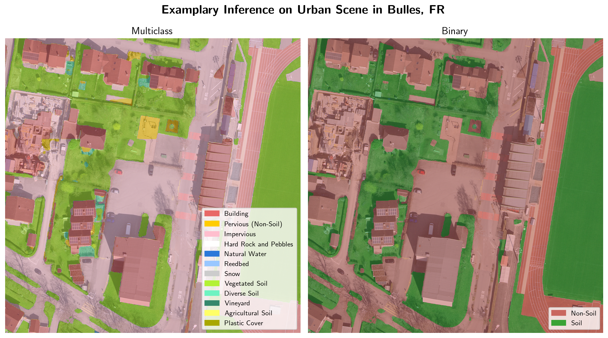
6.3 Examplary Inference

Finally, to show an example of the model output, an inference of the HEIG-VD-mixed-145k model on a 10 cm input resolution tile is given in Figure 28. The inference is a zoomed part in the north-east of the extent shown in Figure 22 and 25. The inference illustrates that the model is capable of distinguishing between different land cover classes in great detail.

Figure 28: Representative inference of the HEIG-VD-mixed-145k model on a 10 cm input resolution tile.

7. Discussion

After presentation of the results, the evaluation and the fine-tuning outcomes are successively discussed.

7.1 Evaluation

All institutions and models have their strengths and weaknesses:

IGN Regarding Extent 1, the model IGN_smp-unet-resnet34-imagenet_RVBI produced the best metrics. Furthermore, the CNN models of IGN are computationally less expensive than the other models and the inferences are not prone to the square artefacts that the HEIG-VD model produces.

HEIG-VD The HEIG-VD model, although it is outperformed by the other two institutions' models on Extent 1, performs significantly better in masked Extent 1 and in Extent 2. The model also performed best in the qualitative assessment. The assessment of the performance in Extent 2 shows that the square artefacts are responsible for a great share of false predictions.

OFS The OFS model OFS_ADELE2(+SAM) performs similarly to the best-performing IGN model, its outputs are not prone to square artefacts, and the inferences are very clean due to its usage of the SAM model. The downside of the OFS model is that it is specifically adapted for the Statistique suisse de la superficie¹⁰ and thus cannot be retrained on a different dataset.

The goal of the evaluation phase was to identify the most promising model for further steps in the project. Based on the results of the evaluation, the HEIG-VD model was chosen. It performed best in masked Extent 1 and in Extent 2, and it performed best in the qualitative assessment. Additionally, the model needs only aerial imagery with the three RGB channels which allows for an easier reproducibility. The model weights and source code of the HEIG-VD model were kindly shared with us, which enabled us to fine-tune the model to adapt to the specifics of this project. However, the premise of choosing the HEIG-VD model was that we are able to mitigate the square artefacts to an acceptable degree.

7.2 Fine-Tuning

The following keypoints can be extracted from the fine-tuning results:

Performance Increase

The fine-tuning procedure could improve the model performance substantially, even though a small dataset was used. For comparison: The FLAIR-1 dataset comprises more than 800 km², which is more than 80 times the size of our used dataset. The improvement is especially impressing, since the chosen model is an attention-based model, which is known to be dependent on large amounts of data ¹⁵. A possible explanation for the success of the fine-tuning is that most of the features that the model has to learn are already present in the pre-trained model. The adjustments of the weights needed to adapt to the specifics of the dataset may, in comparison to the vast amount of information needed to train a model from scratch, be quite small.

Adaptability

Fine-Tuning allows to adjust for different specifics of new datasets. In this case, the model was able to adjust for different resolutions, a different acquisition season, and a new classification scheme. However, also the model that has been trained on the mixed-resolution dataset performed worse on 20 cm and 40 cm resolution input than on 10 cm resolution input. This could be due to the fact that the model has been trained on 4 times as many 10 cm resolution tiles as on 20 cm resolution tiles and 16 times as many 10 cm resolution tiles as on 40 cm resolution tiles. As a result, the model could be biased towards the 10 cm resolution. Another explanation imaginable could be that the defined classes are more easily identifiable in high-resolution input in general. While e.g., the IoU values for the class "sol_vegetalise" does not fluctuate much between the different resolutions, the IoU values for e.g., the class "roche_dure_meuble" seems to depend considerably on the resolution.

Square Artefacts

While a decreased resolution and fine-tuning could not remove the square artefacts completely, their occurence could be drastically reduced. Even more so in the binary case, where the depicted confusion between water and vegetated soil in Figure 27 seems to contribute the most to the square artefacts, which could be reduced by a post-processing step, using known waterbodies as a mask. These water square artefacts that appear by decreasing the resolution, show that the model depends on both resolution and context. Indeed, the lower resolution seems to have removed the specific texture of mountainous meadow and rendered it similar to waterbody. Another factor contributing to this confusion could be a possible bias in the ground truth caused by overrepresented lake sediments that resemble soil.

The resolution decrease affects also the size of the smallest object segmentable. Luckily, urban areas profit the most from high resolution and are not prone to square artefacts, which means that a trade-off could be circumvented by a spatial seperation of high- and low-resolution inferences (e.g., urban: 10 cm, countryside: 40 cm).

7.3 Remarks from Beneficiaries

The beneficiaries provided a feedback of the final state of the model. They were especially content with the performance in heterogeneous areas (i.e., urban areas) and stressed the quality of the inference regarding ambiguous features: the model is able to distinguish between soil and non-soil even in areas where the ground is covered by large objects (e.g., truck trailers), or where the soil is covered by canopies. The model is also not affected by shadows, which was a great concern at the beginning of the project, and shows a good separability of gravel and concrete, which could be used for mapping impervious surfaces. However, the square artefacts are still leading to soil/non-soil confusion, typically appearing as 51.2x51.2m squares in homogeneous areas (with 10 cm resolution). The beneficiaries concluded that around buildings, the soil map produced by the model appears more reliable than other available products and offers the opportunity to cross-reference the binary result (soil – non-soil) with existing indicative maps and to improve the quantitative assessment of the soil concerned by pollutions.

8. Conclusion

One of the main findings of this project is that modern deep learning models are feasible tools to segment various land cover classes on aerial imagery. Furthermore, even complicated models can be fine-tuned for derived specifics and enhanced performance, even in the case of small datasets.

As the mixed-resolution model produces overall better results than the 10cm-only model, it can be considered as the main output of this project. It performs quite well, with an MCC value of 0.938 on the 10 cm validation set. It was able to adapt to the specifics of the Swiss dataset, which incorporates different resolutions, a different acquisition season, and a new classification scheme. The model performs especially well in urban and other high-frequency context areas, where the issue with square artefacts is less pronounced.

The project provides a methodology on how to compare different segmentation models in the geographic domain, gives insights in how a best-suited model can be chosen, and how it can be fine-tuned to adapt to a specific dataset.

8.1 Limitations

The main limitation of this project is the extent of the ground truth data. The ground truth data is only available for a small area in the canton of Fribourg. With a larger dataset, the model may have been able to perform even better and the generalization to other areas may have been better, because each class could have been presented to the model in a more nuanced way.

Another limitation of this project is that the seasonal diversity in the imagery used for this project is very limited. We showed that the model is able to adapt to different vegetation appearances, but the produced model has only been fine-tuned for the vegetation period of the imagery used for training. The model might perform worse in other vegetation periods.

Last but not least, the square artefacts, which were a main concern in the project, still occur within the inferences. The fine-tuning of the model on a mixed-resolution dataset was able to mitigate the effect of the artefacts, but not to remove it completely.

8.2 Outlook

Some ideas that emerged during the project but could not be implemented due to time constraints are:

• As the square artefacts are not much of a problem in urban, high-frequency areas and a lower resolution can help to mitigate the effect of the artefacts in low-frequency, countryside areas, a possible approach could be to infer the model on 10 cm in the urban areas and on 40 cm in the countryside areas. Another way to combine low- and high-resolution inferences could be to make use of an ensemble technique, which combines the predictions of different models to get “the best of both worlds”.

• The confusion between water and vegetated soil is a main cause of error in the binary predictions. A post-processing step to remove these square artefacts could be conducted by using known waterbodies as a mask.

• Another outlook is to conduct further experiments on the effect of the vegetation period on the model performance. This could be done by training the model on different vegetation periods and evaluating it on the same extent.
• Many hyperparameters of the model have been left at their default values that have been set by HEIG-VD. They could be optimized to further increase the model's performance.

8.3 Acknowledgements

We would like to express our gratitude to the people working at HEIG-VD, IGN, and OFS, which contributed significantly to this project by sharing not only their code and models, but also their thoughts and experiences with us. It was a pleasure to collaborate with them.

9. Appendices

Figure 29: Confusion matrix of the HEIG-VD-10cm-71k model on the 10 cm validation set.

Figure 30: Confusion matrix of the HEIG-VD-mixed-145k model on the 10 cm validation set.

Figure 31: Confusion matrix of the HEIG-VD-10cm-71k model on the 20 cm validation set.

Figure 32: Confusion matrix of the HEIG-VD-mixed-145k model on the 20 cm validation set.

Figure 33: Confusion matrix of the HEIG-VD-10cm-71k model on the 40 cm validation set.

Figure 34: Confusion matrix of the HEIG-VD-mixed-145k model on the 40 cm validation set.

Figure 35: Confusion matrix of the original HEIG-VD model on Extent 1.

Figure 36: Confusion matrix of the original HEIG-VD model on Extent 2.

Figure 37: Confusion matrix of the IGN model smp-unet-resnet34-imagenet_RVBI on Extent 1.

Figure 38: Confusion matrix of the IGN model smp-unet-resnet34-imagenet_RVBI on Extent 2.

Figure 39: Confusion matrix of the OFS model OFS_ADELE2(+SAM) on Extent 1.

10. Bibliography

---

1. Pieter Poldervaart and Bundesamt für Umwelt BAFU \textbar Office fédéral de l'environnement OFEV \textbar Ufficio federale dell'ambiente UFAM. Bleibelastung: Schweres Erbe in Gärten und auf Spielplätzen. September 2020. URL: https://www.bafu.admin.ch/bafu/de/home/themen/thema-altlasten/altlasten--dossiers/bleibelastung-schweres-erbe-in-gaerten-und-auf-spielplaetzen.html (visited on 2024-01-04). ↩

2. Christian Niederer. Schwermetallbelastungen in Hausgärten in Freiburgs Altstadt (Kurzfassung), Studie im Auftrag des Amtes für Umwelt des Kantons Freiburg. Technical Report, BMG Engineering AG, 2015. ↩

3. Davide Chicco and Giuseppe Jurman. The advantages of the Matthews correlation coefficient (MCC) over F1 score and accuracy in binary classification evaluation. BMC Genomics, 21(1):6, January 2020. URL: https://doi.org/10.1186/s12864-019-6413-7 (visited on 2024-02-05), doi:10.1186/s12864-019-6413-7. ↩

4. Conseil fédéral suisse. Ordonnance sur les atteintes portées aux sols. 1998. URL: https://www.fedlex.admin.ch/eli/cc/1998/1854_1854_1854/fr. ↩

5. Pavel Iakubovskii. Segmentation Models Pytorch. 2019. Publication Title: GitHub repository. URL: https://github.com/qubvel/segmentation_models.pytorch. ↩

6. Rikiya Yamashita, Mizuho Nishio, Richard Kinh Gian Do, and Kaori Togashi. Convolutional neural networks: an overview and application in radiology. Insights into Imaging, 9(4):611–629, August 2018. Number: 4 Publisher: SpringerOpen. URL: https://insightsimaging.springeropen.com/articles/10.1007/s13244-018-0639-9 (visited on 2024-04-08), doi:10.1007/s13244-018-0639-9. ↩

7. Bowen Cheng, Ishan Misra, Alexander G. Schwing, Alexander Kirillov, and Rohit Girdhar. Masked-attention Mask Transformer for Universal Image Segmentation. June 2022. arXiv:2112.01527 [cs]. URL: http://arxiv.org/abs/2112.01527 (visited on 2024-03-21), doi:10.48550/arXiv.2112.01527. ↩

8. Meng-Hao Guo, Tian-Xing Xu, Jiang-Jiang Liu, Zheng-Ning Liu, Peng-Tao Jiang, Tai-Jiang Mu, Song-Hai Zhang, Ralph R. Martin, Ming-Ming Cheng, and Shi-Min Hu. Attention Mechanisms in Computer Vision: A Survey. Computational Visual Media, 8(3):331–368, September 2022. arXiv:2111.07624 [cs]. URL: http://arxiv.org/abs/2111.07624 (visited on 2024-04-08), doi:10.1007/s41095-022-0271-y. ↩

9. Alexander Kirillov, Eric Mintun, Nikhila Ravi, Hanzi Mao, Chloe Rolland, Laura Gustafson, Tete Xiao, Spencer Whitehead, Alexander C. Berg, Wan-Yen Lo, Piotr Dollár, and Ross Girshick. Segment Anything. April 2023. arXiv:2304.02643 [cs]. URL: http://arxiv.org/abs/2304.02643 (visited on 2024-04-09). ↩

10. Unknown. Arealstatistik Schweiz. Erhebung der Bodennutzung und der Bodenbedeckung. (Ausgabe 2019 / 2020). Number 9406112. Bundesamt für Statistik (BFS), Neuchâtel, September 2019. Backup Publisher: Bundesamt für Statistik (BFS). URL: https://dam-api.bfs.admin.ch/hub/api/dam/assets/9406112/master. ↩↩

11. Zhuang Liu, Hanzi Mao, Chao-Yuan Wu, Christoph Feichtenhofer, Trevor Darrell, and Saining Xie. A ConvNet for the 2020s. March 2022. arXiv:2201.03545 [cs]. URL: http://arxiv.org/abs/2201.03545 (visited on 2024-03-21), doi:10.48550/arXiv.2201.03545. ↩

12. Dirk Merkel. Docker: lightweight linux containers for consistent development and deployment. Linux journal, 2014(239):2, 2014. ↩

13. Adam Paszke, Sam Gross, Francisco Massa, Adam Lerer, James Bradbury, Gregory Chanan, Trevor Killeen, Zeming Lin, Natalia Gimelshein, Luca Antiga, Alban Desmaison, Andreas Köpf, Edward Yang, Zach DeVito, Martin Raison, Alykhan Tejani, Sasank Chilamkurthy, Benoit Steiner, Lu Fang, Junjie Bai, and Soumith Chintala. PyTorch: An Imperative Style, High-Performance Deep Learning Library. December 2019. arXiv:1912.01703 [cs, stat]. URL: http://arxiv.org/abs/1912.01703 (visited on 2024-04-02), doi:10.48550/arXiv.1912.01703. ↩

14. MMSegmentation Contributors. MMSegmentation: OpenMMLab Semantic Segmentation Toolbox and Benchmark. 2020. URL: https://github.com/open-mmlab/mmsegmentation. ↩↩

15. Abdul Mueed Hafiz, Shabir Ahmad Parah, and Rouf Ul Alam Bhat. Attention mechanisms and deep learning for machine vision: A survey of the state of the art. June 2021. arXiv:2106.07550 [cs]. URL: http://arxiv.org/abs/2106.07550 (visited on 2024-04-09). ↩